6. Sequential Logic
Most of today’s digital systems are build with sequential logic, including virtually all computer systems. A sequential circuit is a digital circuit whose outputs depend on the history of its inputs. Thus, sequential circuits have a memory that permits significantly more complex functional behaviors than combinational circuits are capable of. In fact, the study of the complexity of sequential circuit behavior is the cradle of the field of computer science.
6.1. Feedback Loops
We construct a sequential circuit by introducing a feedback loop. For example, we may connect the output of a combinational circuit to one of its inputs, as shown in Figure 6.1. This multiplexer circuit feeds output \(Y\) back to data input \(D_0.\) Because of this feedback loop, inputs of the past, in particular inputs that are arbitrarily older than the propagation delay of the multiplexer, can determine output \(Y.\) In the following, we analyze the circuit to derive a precise characterization of its behavior.

Figure 6.1: Multiplexer with feedback loop (left), and glitch-free implementation with consensus term \(X\) (right).
We may express the functionality of the multiplexer loop by means of the defining equation of the multiplexer, substituting \(Y\) for data input \(D_0\) and \(D\) for data input \(D_1\):
This definition is recursive, because \(Y\) appears as output on the lhs and as input on the rhs in case \(S=0.\) We interpret the recursion such that output \(Y\) follows input \(D\) if select input \(S\) equals 1, and holds output \(Y\) while \(S\) equals 0. Thus, when \(S=0\) the circuit retains the last value of input \(D\) before \(S\) transitions from 1 to 0. We know this behavior from the D-latch already. Now, we utilize the tools for combinational circuit design, including K-maps and timing analysis, to study the feedback loop in more detail.
First, we inspect the combinational portion of the multiplexer circuit without the feedback loop, and second we study the effects of the feedback loop. This separation of concerns is known as cut analysis:
- Cut all feedback loops, and rename all fed-back outputs that drive the loops.
- Analyze the combinational circuit by deriving the K-maps, called excitation table, for each fed-back output.
- Generate the transition table by marking all stable states in the excitation table, i.e. those K-map cells where the outputs driving the feedback loops equal the inputs driven by the feedback loops.
- Analyze the transitions of the sequential circuit in the presence of all feedback loops with the aid of the transition table.
We analyze the multiplexer circuit, starting with step 1 by cutting the feedback loop. Figure 6.2 illustrates the cut in the black-box diagram on the left and the combinational circuit implementing a glitch-free multiplexer on the right. We rename output \(Y\) that drives the feedback loop to \(Y',\) and keep name \(Y\) for the input of the multiplexer that is driven by the feedback loop.

Figure 6.2: Step 1 of cut analysis: cut the feedback loop, keep combinational input name \(Y,\) and rename the combinational output into \(Y'.\)
The resulting gate-level circuit of the multiplexer in Figure 6.2 is acyclic and, hence, combinational. Output \(Y'\) is a function of three inputs, \(D,\) \(S,\) and \(Y\):
The equivalent SOP form corresponding to the gate-level circuit is
Besides analyzing the functionality, we can analyze the timing of the combinational circuit, which resembles the analysis of the multiplexer without consensus term. Assume for simplicity that each gate has a propagation delay of 1 time unit, i.e. \(t_{pd}(inv) = 1,\) \(t_{pd}(and) = 1,\) and \(t_{pd}(or) = 1.\) Then, the multiplexer in Figure 6.2 has one path from \(S\) through the inverter with propagation delay \(t_{pd}(mux) = 3\) time units, and all other paths have contamination delay \(t_{cd}(mux) = 2\) time units. This completes our analysis of the combinational circuit.
According to step 2 of the cut analysis, we translate the multiplexer function into a K-map, also called excitation table, because it specifies the function of the circuit node that drives or excites the feedback loop. In case of the multiplexer circuit this node is \(Y'.\) Figure 6.3 shows the excitation table of \(Y'\) on the left. We have arranged variable \(Y\) to change across rows, because this simplifies step 3, determining the stable states for the transition table.

Figure 6.3: Excitation table (left) and transition table (right) of the multiplexer loop.
A circuit with a feedback loop is stable, if the output of the combinational circuit that drives the feedback loop is equal to the input of the combinational circuit driven by the feedback loop. After all, this is the purpose of the feedback wire to begin with: The feedback wire forces the voltage levels of the connected output and input of the combinational circuit to be equal. The stable states of our multiplexer loop are those cells in the excitation table where output \(Y'\) equals input \(Y.\) In Figure 6.3, the top row is associated with input \(Y=0.\) Therefore, the stable states are those cells of the top row marked with \(Y' = 0.\) Analogously, the bottom row is associated with \(Y=1,\) such that the stable states in the bottom row are all cells marked with \(Y' = 1.\) The excitation table with encircled cells identifying stable states is called transition table, see Figure 6.3 on the right. All remaining cells without circle identify unstable states. An unstable state is temporary, because output \(Y' \ne Y\) drives a new input \(Y'\) via the feedback loop into the combinational circuit.
We now use the transition table to pursue our original goal, the systematic analysis of the transitions of the multiplexer loop, i.e. step 4 of the cut analysis. The input terminals of the multiplexer loop in Figure 6.1 are data input \(D\) and select input \(S.\) We assume that the circuit is in a stable state, for example \((D,S,Y) = 100.\) This is the state associated the rightmost cell in the top row of the transition table, shown on the left in Figure 6.4 below. The loop holds output value \(Y' = 0\) indefinitely until we stimulate a transition by changing an input.

Figure 6.4: Transition paths of multiplexer loop stimulated by input change \(S: 0 \rightarrow 1\) (left) and then \(D: 1 \rightarrow 0\) (right).
Next, we change select input \(S\) from 0 to 1. In the transition table, we move by one cell to the left. This state is unstable, because output \(Y'=1\) differs from input \(Y=0.\) Input \(Y\) will assume output value 1 via the feedback loop after a delay of \(t_{cd} = 2\) time units, because inputs \((D,S)=11\) cause AND gate \(W\) to change from 0 to 1, which switches output \(Y'\) from 0 to 1. Therefore, the circuit transitions without further stimulus from unstable state \((D,S,Y)=110\) to state \((D,S,Y)=111.\) In the transition table, we move by one cell downward. State \((D,S,Y)=111\) is stable and produces output \(Y'=1.\) The same transition behavior occurs in a D-latch, after switching from opaque to transparent. The output follows input \(D\) such that \(Y'\) transitions from 0 to 1.
If we change data input \(D\) from 1 to 0 when the multiplexer loop occupies stable state \((D,S,Y)=111,\) the state transitions along the path illustrated in Figure 6.4 on the right. Since \((D,S,Y)=011\) is an unstable state, input \(Y\) will change to output \(Y'=0.\) Without further stimulus the circuit transitions to stable state \((D,S,Y)=010.\) The transition table enables us to argue about such transitions without inspecting the circuit diagram. Thus, the transition table is a powerful tool suited for tracing all possible transition paths in a circuit with feedback loops. In the transition table of the multiplexer loop, signal changes on the input terminals \(D\) or \(S\) correspond to transitions across columns within a row. State transitions due to the feedback loop start in an unstable state and cross rows within a column.
The transition table can be viewed as a simplifying abstraction of the timing diagram resulting from a timing analysis. The waveforms of the timing diagram provide the delays as additional information. Figure 6.5 shows the timing diagram of the transitions discussed in Figure 6.4 based on the signals of the multiplexer loop in Figure 6.1. Input transition \(S: 0 \rightarrow 1\) occurs at time \(t = 0,\) and input transition \(D: 1\rightarrow 0\) at time \(t = 6.\) Since we assume that each gate has a delay of 1 time unit, the transition of select input \(S\) takes a delay of \(t_{cd} = 2\) time units to produce a stable output \(Y=1,\) although it takes another time unit for the feedback loop to drive node \(X\) to value 1. Similarly, the transition of data input \(D\) takes \(t_{cd} = 2\) time units stabilize output \(Y=0.\)

Comparing the timing diagram with the transition tables in Figure 6.4, we observe that the multiplexer loop is in initial state \((D,S,Y)=100\) for \(t < 0.\) Then, we change select input \(S\) to 1, and the circuit is in unstable state \((D,S,Y)=110\) for time period \(0 < t < 2.\) At time \(t=2,\) output \(Y\) transitions to 1, and the circuit into stable state \((D,S,Y)=111.\) The multiplexer loop remains in this state until we provide the next input stimulus. This happens at time \(t=6,\) where we change data input \(D\) to 0. In time period \(6 < t < 8,\) the circuit occupies unstable state \((D,S,Y)=011,\) before it transitions into stable state \((D,S,Y)=010\) at time \(t=8.\) The transition table captures these transitions without the complexity of a timing analysis.
Using the transition table, we can study the behavior of the multiplexer loop when select input \(S = 0.\) Figure 6.6 shows on the left the transition starting in state \((D,S,Y)=010\) and changing \(S\) from 1 to 0. We move by one cell to the left into stable state \((D,S,Y)=000.\) Subsequently, we can change data input \(D\) from 0 to 1, transitioning the circuit to stable state \((D,S,Y)=100,\) and back, as shown in Figure 6.6 on the right. Output \(Y\) stores the last value of \(D,\) before we changed \(S\) from 1 to 0, no matter when and how often we toggle data input \(D.\) This timing behavior demonstrates the characteristic feature of sequential circuits: ouput \(Y\) depends on the history of inputs \(D\) and \(S.\) If \(D\) would have been 1 before we changed \(S\) from 1 to 0, the multiplier loop would have stored \(D=1\) by holding output \(Y = 1\) in stable states \((D,S,Y)=101\) or \((D,S,Y)=001.\)

Figure 6.6: Transition paths of multiplexer loop stimulated by input change \(S: 1 \rightarrow 0\) (left) and subsequently toggling \(D\) (right).
The distinction of stable and unstable states leads us to classify the behavior of entire sequential circuits with feedback as either stable or unstable. A sequential circuit is stable, if a change at an input terminal causes the circuit to transition from one stable state into another. Otherwise, if the outputs change beyond the propagation delay, the sequential circuit is unstable. We distinguish two types of unstable circuit. If the outputs become stable eventually, then the change of an input causes the circuit to transition through one or more unstable states into a stable state. If, however, the outputs change indefinitely, then the circuit must enter a cycle of transitions through unstable states. Unless we wish to design an oscillator, such a behavior is usually considered a bug. Transitions that are eventually stable but traverse unstable states are considered a harmless feature of sequential circuits, similar to glitches in combinational circuits.
We perform a cut analysis of the ring oscillator in Figure 6.7. The feedback loop connects output \(Y\) to the input of the NAND gate. We cut the feedback loop and rename output \(Y\) to \(Y'.\)

Figure 6.7: Ring oscillator with control input \(A\) and cut through feedback loop.
The combinational portion of the cyclic circuit is the 3-stage path NAND-INV-INV. The output function \(Y'(A,Y)\) is easily derived as follows. Since \(Y' = \overline{X} = W,\) we find \(Y' = \overline{A \cdot Y}.\) We may interpret the function of the NAND gate as
such that output \(Y'\) equals 1 if control input \(A=0,\) and \(Y'\) is the complement of input \(Y\) if \(A=1.\) Next, we translate this functionality into a K-map, and encircle the only stable state \((A,Y)=01\) to obtain the transition table below.

Based on the transition table we deduce the behavior of the ring oscillator. If input \(A=0,\) the circuit will eventually enter the stable state. If the circuit is in unstable state \((A,Y)=00,\) then output \(Y'=1\) enforces the transition into stable state \((A,Y)=01.\) If we change input \(A\) from 0 to 1, we move from the stable state by one cell to the right. State \((A,Y)=11\) is unstable. Since \(Y' = 0,\) it transitions after the propagation delay of the 3-stage path to state \((A,Y)=10,\) i.e. we move one cell up in the transition table. The resulting state \((A,Y)=10\) is unstable too. Output \(Y'=1\) forces the transition to state \((A,Y)=11,\) i.e. we move one cell down again. As long as input \(A\) remains 1, the circuit toggles between states \((A,Y)=10\) and \((A,Y)=11,\) and the output between \(Y'=0\) and \(Y'=1.\) The propagation delay between transitions is the delay of the 3-stage path. In other words, the oscillator produces a clock signal. To stop the oscillation, we change input \(A\) from 1 to 0, so that the circuit transitions into the stable state eventually. In the transition table, stimulus \(A: 1\rightarrow 0\) moves from the right to the left column, and if we are in the top row, then without further stimulus into the bottom row.
Not all combinational circuits with a feedback loop are sequential. There exist cyclic circuits whose outputs depend on the present inputs only rather than on the past inputs. An example of such a multioutput circuit is shown below.

We use a modified form of the cut analysis to show that this circuit is combinational. A circuit is sequential if we cut the feedback loop and the output driving the feedback loop is a function of the inputs driven by the feedback loop. If the output function of the driver of the feedback loop is independent of the feedback signal, then the feedback wire is redundant and the circuit is combinational.
Following this argument, we investigate whether output \(y_3\) of the circuit is sequential or combinational. We cut the feedback loop as shown below, and rename the output into \(y_3'.\)

Next, we deduce the Boolean expression for \(y_3'\) as a function of inputs \(x_0,\) \(x_1,\) and feedback input \(y_3,\) and simplify the expression to see whether \(y_3'\) depends on \(y_3\) or not:
We conclude that \(y_3'\) is not a function of feedback input \(y_3\) but is a function of terminal inputs \(x_0\) and \(x_1\) only. Therefore, \(y_3'\) depends on the present inputs \(x_0\) and \(x_1\) only, and is hence combinational.
Since the circuit is a multioutput circuit, it is combinational if all of its output functions are combinational. Therefore, we repeat the cut analysis for each output, cutting the loop at the input driven by the corresponding output. For example, to test \(y_0,\) we cut the loop at the \(y_0\)-input of the AND gate. Then, we find these expressions for the output functions:
None of the output functions depends on the feedback signal. Therefore, all output functions and the circuit as a whole are combinational. Intuitively, the complementation and covering theorems cause the feedback signal to vanish from the outputs. More interesting is the observation that this cyclic combinational circuit computes four distinct 2-variable functions with four gates, and is therefore competitive with four independent acyclic circuits.
Perform a cut analysis of the NAND loop:

- Cut the loop and rename the loop driver.
- Derive a K-map for the output (excitation table).
- Mark all cells with stable states (transition table).
- Analyze the transitions of the circuit.
Output \(Y\) of the NAND gate drives the feedback loop to its input. The first step of a cut analysis is to cut the feedback loop:

Then, we rename the loop driver, here \(Y \rightarrow Y',\) and redraw the resulting acyclic combinational circuit to enhance clarity:

The combinational circuit in (b) is easy to analyze: \(Y' = \overline{A\,Y}.\)
The excitation table of the loop circuit is the K-map of the acyclic combinational circuit, specified above by means of Boolean equation \(Y' = \overline{A\,Y}.\) Since the NAND operation produces \(Y' = 0\) only if both inputs are \(A = Y = 1,\) the corresponding K-map is:

We derive the transition table of the cyclic circuit with feedback loop from the excitation table of the acyclic circuit by marking all stable states that observe feedback constraint \(Y = Y'.\) The cells of the excitation table are marked with the associated value of output \(Y'.\) In the top row of the excitation table input \(Y = 0.\) However, both cells are marked with output \(Y' = 1.\) Thus, there are no stable states in the top row. In the bottom row of the excitation table input \(Y = 1.\) The leftmost cell is marked with output \(Y' = 1,\) which is equal to input \(Y.\) Therefore, this cell identifies the only stable state of the circuit.

We study the transitions of the NAND loop with the aid of the transition table. Input \(A\) is the only input of the NAND loop. Therefore, we first study the behavior of the circuit when \(A\) is fixed either to 0 or to 1, and then when input \(A\) changes.
Consider the case where input \(A = 0.\) We distinguish two cases depending on input \(Y.\) If \(Y = 1\) initially, then the circuit is in its stable state because output \(Y' = \overline{0\cdot 1} = 1\) of the NAND gate reinforces input \(Y = Y' = 1\) through the feedback loop. In the other case, input \(Y = 0\) initially. In the transition table below this initial state is associated with the top-left cell where \((A,Y) = 00.\)

State \((A,Y)=00\) is unstable, because output \(Y'=1\) of the NAND gate drives input \(Y=Y'=1\) through the feedback loop, which differs from the initial state \(Y=0.\) Thus, the feedback loop transitions the circuit into new state \((A,Y)=01.\) This is the stable state of the circuit associated with the bottom-left cell. After transitioning into the stable state, the circuit has stabilized. We conclude that the circuit stabilizes when input \(A=0\) such that output \(Y'=1\) eventually.
Next, we consider case \(A=1.\) If input \(Y=0\) initially, the circuit is in state \((A,Y)=10\) associated with the top-right cell of the transition table. Since the output of the NAND gate produces \(Y'=1,\) the feedback loop enforces the input transition \(Y: 0\rightarrow 1.\) The circuit transitions to state \((A,Y)=11\) associated with the bottom-right cell of the transition table.

In the other case, where input \(Y=1\) initially, the circuit is in state \((A,Y)=11.\) This state is unstable, because output \(Y'=0\) of the NAND gate enforces the input transition \(Y: 1\rightarrow 0\) through the feedback loop. Thus, the circuit transitions to state \((A,Y)=10.\) We conclude that the circuit oscillates when input \(A=1,\) like the ring oscillator of Example 6.1.
Changes at input \(A\) transition the circuit between stable state \((A,Y) = 01\) and the oscillating behavior when input \(A=1.\) The exact state sequence of the transition depends on the state of the circuit when \(A\) transitions. In particular, if the circuit oscillates when \(A\) changes from 1 to 0, input \(Y\) assumes one of the two values 0 or 1 beyond our control. If \(Y\) happens to be 1, then state transition \((A,Y): 11 \rightarrow 01\) assumes the stable state immediately. On the other hand, if \(Y\) happens to be 0 when \(A\) changes from 1 to 0, then the state transitions through unstable state 00 into stable state 01, i.e. \((A,Y): 10 \rightarrow 00 \rightarrow 01.\) The inverse input transition \(A: 0\rightarrow 1\) causes the circuit to oscillate, most likely originating in stable state \((A,Y) = 01,\) because unstable state \((A,Y)=00\) transitions into the stable state when \(A=0.\)
6.2. Synchronous Circuits
Feedback is the key to processing past and present information of an input sequence. Memory elements, including the D-latch and the D-flipflop, are sequential circuits with feedback loops. In general, it is nontrivial to design a sequential circuit by augmenting a combinational circuit with feedback loops, because the delays of such loops are difficult to control and the timing behavior of compositions is hard to analyze. Even worse, hazards are difficult to predict in compositions of subcircuits with feedback loops, and potentially cause the circuit to become unstable indefinitely and malfunction. Nevertheless, sequential circuits with feedback loops are of interest per se, and design methodologies have been developed to cope with the problems of this class of circuits, widely known as asynchronous circuits today. The D-latch and the D-flipflop are asynchronous sequential circuits whose design has benefited from these developments.
Another circuit style dominates today’s digital design practice, known as synchronous circuits. The name derives from the introduction of a chronometer or clock signal that is used to trigger all D-flipflops of a circuit at the same beat of the clock. Furthermore, in an effort to simplify the control of delays through feedback loops, we insert a D-flipflop in every feedback loop. Since D-flipflops are edge-triggered memory elements, their outputs are stable for an entire clock period. When placed in a feedback loop, the output of the D-flipflop is the feedback input for the combinational circuit. Other than in an asynchronous circuit, the D-flipflop keeps the feedback input stable during the clock period. Hence, the loop cannot become unstable and can even tolerate hazards in the combinational logic, provided the clock period is larger than the combinational propagation delay.
The design style of synchronous circuits radically restricts the overall design space for sequential circuits. Nevertheless, it simplifies the task of circuit design dramatically, and is still powerful enough to assemble reliable circuits with billions of transistors. As such the synchronous design style is part of the unique success story of large scale digital systems engineering. Given their practical importance, we focus the remainder of this chapter on synchronous sequential circuits. This section discusses an analysis methodology for synchronous sequential circuits and introduces three sequential building blocks, a binary counter, shift registers, and memories.
6.2.1. Analysis of Synchronous Sequential Circuits
We demonstrate the functional analysis of synchronous sequential circuits by means of the multiplexer loop, extended with a D-flipflop in the feedback loop. As shown in Figure 6.8, D-flipflop output \(Q\) drives the feedback input of the multiplexer, and clock signal \(\phi\) triggers the D-flipflop at the positive clock edge. At this point in time the D-flipflop stores its input \(Y\) for an entire clock cycle until the next positive clock edge occurs.

Figure 6.8: Multiplexer with D-flipflop in feedback loop triggered by clock signal \(\phi.\)
The value stored in the D-flipflop is called the state of the synchronous circuit. In Figure 6.8 the state is observable at D-flipflop output \(Q.\) The purpose of circuit analysis is to determine the next state of the next clock cycle. If we consider all possible input combinations, the analysis enables us to predict the sequence of output values given a sequence of input values. The next state of the multiplexer loop is the value of input \(Y\) of the D-flipflop at the time of the triggering clock edge. Signal \(Y\) is driven by the combinational multiplexer circuit, and is a function of inputs \(D\) and \(S,\) and state \(Q\):
We use an adapted form of transition table, the so-called state transition table, to list the next state as a function of the state and the inputs. Since the state of the circuit is equal to \(Q\) and the next state is equal to \(Y,\) the state transition table of the multiplexer loop in Figure 6.8 is:
state (\(Q\)) \(D\) \(S\) next state (\(Y\)) 0 0 0 0 0 0 1 0 0 1 0 0 0 1 1 1 1 0 0 1 1 0 1 0 1 1 0 1 1 1 1 1
State transition tables are commonly drawn in form of a truth table, although we could use the equivalent K-map form as well. Under the assumption that the input values \(D\) and \(S\) are stable at the time of the triggering clock edge, we derive next state \(Y\) by evaluating equation \(Y(D,S,Q)\) for the combination of input values in each row. This equation specifies the next state logic implemented by the combinational multiplexer.
Although the state transition table specifies the transition behavior of a sequential circuit unambiguously, it can be advantageous to visualize the transition behavior by means of a directed graph, the so-called state transition diagram. Here, each vertex represents a state, and each arc a transition. We annotate the arcs with the combination of input values associated with the state transition. Separated by a slash, we also include output \(Y\) of the circuit, which happens to be equal to the next state in this example. Figure 6.9 shows the state transition diagram of the multiplexer loop in Figure 6.8. The vertices are marked with the value of state \(Q.\) The format of the arc annotations is \((D,S)/Y,\) i.e. the pair of input values followed by a slash followed by the output value.

Figure 6.9: State transition diagram of synchronous multiplexer loop. Arcs are marked with input and output values, separated by a slash.
We interpret the state transition diagram as follows. During the present clock cycle, the circuit is in one of the states represented by a vertex, for example in state 0. While in this state, the inputs may change causing the output to change. For example, in state 0, if we apply inputs \((D,S)=01,\) then output \(Y=0,\) as indicated by arc annotation \(01/0.\) If we apply inputs \((D,S)=11,\) then output \(Y=1,\) and the arc annotation is \(11/1.\) The input combination at the time of the triggering clock edge determines the next state. For example, arc \(11/1\) points from state 0 to state 1, because at the triggering clock edge next state \(Y=1\) is stored in the D-flipflop. The other three input combinations \(00/0,\) \(01/0,\) and \(10/0\) store next state \(Y=0\) at the triggering clock edge, which is also the present state. Therefore, the corresponding arc is a loop from state 0 to state 0 for all three input combinations. Comparison with the next state table shows that each arc annotation in the diagram corresponds to one row in the table. The diagram captures the transition behavior in a more compact form, that some designers find easier to comprehend than a table.
The state transition table and/or the state transition diagram enable us to derive the output sequence of the circuit if the inputs are synchronized with the clock, such that during each clock cycle one new pair of inputs arrive. For example, assume that the multiplexer loop is initially in state 0, and we apply the input sequence 00, 11, 10, 01, 10. Then, the corresponding output sequence is 0, 1, 1, 0, 0. Here is why. Initially, the circuit is in state 0, and we apply the first input pair 00. Hence, the output is \(Y=0.\) At the next triggering clock edge, the D-flipflop stores next state 0. Now, we apply the second input pair 11. The output changes to \(Y=1.\) At the next triggering clock edge the circuit transitions to state 1. The third input pair 10 holds output \(Y=1,\) and so on. Use the interactive model in Figure 6.10 to develop a feeling for the synchronous multiplexer loop. You can toggle inputs \(D\) and \(S\) and trigger a positive clock edge by pushing the \(\phi\) trigger button.
D = 0 S = 0 Figure 6.10: Interactive model of synchronous multiplexer loop.
The multiplexer loop does not restrict the inputs to change only once per cycle. In fact, you can change inputs \(D\) and \(S\) as often as you like between triggering clock edges. The output follows the inputs through the combinational logic implemented by the multiplexer. State changes, however, occur only upon triggering a positive clock edge. At this time, the D-flipflop stores the next state supplied to its input by multiplexer output \(Y.\) In summary, if input \(S=1,\) the loop stores input \(D\) at the time of the clock trigger. Otherwise, while \(S=0,\) the loop holds its state across clock trigger events independent of \(D.\) The state transition table and diagram above contain the same information about the circuit.
In the following, we analyze several synchronous sequential circuits by deriving their state transition table and diagram. These circuits are sequential building blocks for the design of larger sequential circuits.
6.2.2. Binary Counter
An \(n\)-bit binary counter is a synchronous sequential circuit that increments its \(n\)-bit output \(Y\) at every triggering clock edge. Since \(n\) bits can represent unsigned numbers in range \([0, 2^n-1],\) the counter rolls over to 0 when incrementing the largest value \(2^n-1\) of the representable number range. Therefore, \(n\)-bit binary counters are also called modulo-\(2^n\) counters. Figure 6.11 shows a 3-bit binary counter with a reset input to force the counter to zero. While the reset input is 0, the reset signal is inactive. Whenever a positive clock edge occurs the counter increments the value stored in the 3-bit register. If the reset input is equal to 1 during a positive clock edge, the register is reset to zero.
reset = 0 Figure 6.11: Interactive model of a 3-bit binary counter.
The counter circuit is synchronous, because the feedback loop contains a clock triggered register. Output \(Y\) of the register feeds back into the 3-bit adder. The second input of the adder is hardwired to constant value \(1_{10}.\) We tacitly assume that the carry-in of the adder is grounded to value 0, and the carry-out is unused. Sum output \(S\) of the adder generates the 3-bit sum \(S=(Y+1) \bmod 8.\) Recall that the largest unsigned binary number representable with 3 bits is \(2^3-1 = 7_{10},\) and \(7+1=8_{10} = 1000_2\) requires 4 bits. Since the sum output of the adder excludes the most significant carry-out bit, we obtain \(S = 000_2 = 0_{10}\) for input \(Y=7_{10}.\) The multiplexer implements the reset logic. Next state signal \(Y'\) is the output of the combinational portion of the feedback loop, and obeys the multiplexer logic:
We analyze the behavior of the counter circuit by deriving the state transition diagram. The circuit has one input besides clock \(\phi,\) i.e. the reset signal, and one output, which is counter value \(Y.\) First assume that the reset signal is inactive, and the counter increments its output at every positive clock edge. During a clock cycle the register stores the present state and drives it on output \(Y,\) where we can observe the state. At the next positive clock edge, the circuit transitions to next state \(Y'.\) We draw the state transition diagram, we need to start with some state, for example state \(0_{10}.\) We represent the state with a new vertex and mark it with its identifying state value 0. The next state of state \(0_{10}\) is \(Y'=1_{10}.\) We draw a second vertex, mark it with state value \(1_{10},\) and draw an arc from vertex 0 to vertex 1.

Figure 6.12: State transition diagram of 3-bit binary counter. Arcs are marked with input values only. Vertices are augmented with the output values.
Rather than annotating the arc with the output value as we did in Figure 6.9, we annotate the vertices with the output values. The reason for this change is a subtle difference in the output behavior of the circuits. In the multiplexer loop of Figure 6.8 the combinational logic drives the output whereas in the counter loop of Figure 6.11 the register drives the output. Whereas the output of the multiplexer loop depends on the present inputs, this is not the case for the binary counter. Output \(Y\) of the binary counter is stable during the entire clock cycle, independent of the reset input. The output changes only at the positive clock edge. In the state transition diagram in Figure 6.12 we emphasize this behavior by marking arcs with the input value of the reset input, and augment the state vertices with the output value.
As long as the reset input is 0, the counter circuit transitions from state \(Y\) to state \((Y+1) \bmod 8\) at each triggering clock edge. Thus, the state transition graph is a single cycle with eight states. If the reset input is 1, however, the counter transitions to state 0, independent of the present state. The reset arcs form additional cycles in the state transition diagram. As shown in Figure 6.12, the complete diagram has nine cycles. We could join the output arcs of state 7, however, because both input values 0 and 1 cause a transition to state 0.
The state transition table is the equivalent representation of the state transition diagram in Figure 6.12. For the binary counter, it assumes the form of a truth table with one column for the present state and the reset signal as inputs, and the next state as output. Frequently, designers augment the state transition table with the output specification, here with one column for output \(Y\):
state reset next state output 0 0 1 0 0 1 0 0 1 0 2 1 1 1 0 1 2 0 3 2 2 1 0 2 3 0 4 3 3 1 0 3 4 0 5 4 4 1 0 4 5 0 6 5 5 1 0 5 6 0 7 6 6 1 0 6 7 0 0 7 7 1 0 7
In case of the binary counter, specifying output \(Y\) in the state transition diagram or table is redundant, since the state and the output are equal. This is not the case in general, however. Note that we can deduce from the state transition table that the output is driven by the register rather than the combinational logic, because the output equals the present state, independent of the reset input.
6.2.3. Shift Register
An \(n\)-bit shift register has one serial input and \(n\) parallel outputs. Its function can be described as a serial-to-parallel converter. Figure 6.13 shows a 4-bit shift register with serial input \(S_{in}\) and four parallel outputs \(Y_i,\) where \(0 \le i < 4.\) Some implementations provide parallel output \(Y_{n-1}\) also as a separate serial output \(S_{out}.\) At each positive clock edge, the state is shifted by one D-flipflop to the right. After shifting four bits during four consecutive clock cycles into the shift register, all four bits are available at the parallel outputs. Considering the serial input and serial output only, the shift register implements a FIFO, short for first-in-first-out buffer. The first of multiple bits shifted in at \(S_{in}\) is the first bit to be shifted out at \(S_{out}.\) It takes four clock cycles for a bit to propagate through the FIFO.
Sin = 0 Figure 6.13: Interactive model of a 4-bit shift register.
The shift register is a synchronous sequential circuit, although the circuit diagram does not show any loops. The feedback loops are hidden inside the D-flipflops. In essence, a shift register is a series composition of D-flipflops, all triggered by the same clock signal. The state of the shift register can be observed at the outputs as binary number \(Y_3 Y_2 Y_1 Y_0.\) Figure 6.13 enables you to derive the state transition table of the 4-bit shift register:
state \(S_{in}\) next state output 0 0 0 0000 0 1 8 0000 1 0 0 0001 1 1 8 0001 2 0 1 0010 2 1 9 0010 3 0 1 0011 3 1 9 0011 4 0 2 0100 4 1 10 0100 5 0 2 0101 5 1 10 0101 6 0 3 0110 6 1 11 0110 7 0 3 0111 7 1 11 0111 8 0 4 1000 8 1 12 1000 9 0 4 1001 9 1 12 1001 10 0 5 1010 10 1 13 1010 11 0 5 1011 11 1 13 1011 12 0 6 1100 12 1 14 1100 13 0 6 1101 13 1 14 1101 14 0 7 1110 14 1 15 1110 15 0 7 1111 15 1 15 1111
The state transition table confirms that the outputs are independent of input \(S_{in}.\) This is no surprise, because the outputs are driven by the D-flipflops. Besides, the shift register has no combinational logic other than wires. Therefore, when drawing the corresponding state transition diagram we associate the output with a state vertex and the value of input \(S_{in}\) with an arc, analogous to the state transition diagram of the binary counter in Figure 6.12. We leave it as an exercise to translate the state transition table into a state transition diagram. You may view the resulting state transition diagram as a directed graph, and find the shortest paths to transition from one state to another in order to minimize the number of clock cycles and the length of the serial input sequence. For example, given state 6 you need at least two cycles to transition to state 9. The path transitions through state 3 by first applying serial input 0 and then 1.
We can extend the shift register to function not only as a serial-to-parallel converter but also as a parallel-to-serial converter. To that end, we provide parallel data inputs and include a multiplexer at each D-flipflop input. Figure 6.14 shows the extended 4-bit shift register. The Load input selects the multiplexer inputs between the parallel data inputs \(D_i,\) \(0 \le i < 4,\) and the original serial inputs. When Load equals 1 at the triggering clock edge, all D-flipflops store the values provided at the parallel data inputs. Otherwise, when Load equals 0, the circuit performs a right shift. During each clock cycle, the circuit outputs the data serially, bit-by-bit, at output \(S_{out}.\)

Figure 6.14: 4-bit shift register with parallel load.
The shift register in Figure 6.14 can be used to implement the ports of a serial communication channel, such as RS-232. The sender uses the parallel-to-serial functionality to load a byte of data into the shift register, and transmit the byte serially across one wire to a receiver. The receiver shifts the bits serially into its shift register, and outputs the byte in parallel, using the serial-to-parallel functionality.
6.2.4. Memories
The memory elements discussed so far, including the D-flipflop, are relatively fast circuits but require more transistors than necessary to store a single bit. The hallmark of memory circuits is their density, i.e. the number of bits stored per unit of chip area.
Memory Organization
There exist serveral different technologies to implement a 1-bit memory element. However, independent of the technology virtually all memory architectures consist of a 2-dimensional array of such 1-bit memory elements, also called bit cells in this context. Figure 6.15 shows the block diagram of a \(4\times 3\) array of bit cells.

Figure 6.15: Memory array with 4 rows and 3 columns of bit cells.
The array has an address bus \(A\) as input, and a data bus \(D\) as input and output. In general, \(n\)-bit address \(A\) drives an \(n{:}2^n\)-decoder to assert one of \(2^n\) wordlines, thereby selecting one row of the array of bit cells. We call a group of \(m\) data bits a word, and consider a word the unit of data transfer in and out of the memory array. In order to read one word out of one row of bit cells, we apply the associated binary-coded address, and the \(m\)-bit data bus outputs the word via the bitlines. If we want to write a word into the memory, we drive the word onto the bitlines, and apply the desired address.
Each bit cell is responsible for implementing a tristate behavior depending on the select input driven by the wordline and the signal on the bitline. Figure 6.16 shows one bit cell with its select input \(S\) connected to the wordline and data port \(D\) connected to the bitline for input and output. If the wordline drives a 0 on select input \(S,\) the cell disables data port \(D,\) indicated by value \(Z\) in Figure 6.16. As a result the cell is invisible to the bitline. Otherwise, if the wordline drives a 1 on select input \(S\) the cell is enabled. The enabled cell performs a read or write operation depending on the state of the bitline. In order to write the cell, we use a tristate buffer to drive the desired value onto the bitline. This data input is enabled with signal \(D_{en}.\) While \(D_{en} = 1,\) the tristate buffer drives data input \(D_{in}\) onto the bitline, and writes \(D_{in}\) into the enabled cell. On the other hand, if \(D_{en}=0,\) the data input is disabled, and the enabled cell makes its stored bit visible to the bitline, where we can observe it at data output \(D_{out}.\)
wordline = 0 Den = 0 Din = 0 Figure 6.16: Interactive model for reading and writing a bit cell.
When multiple rows of bit cells are arranged in an array, all cells in a column are connected to the same bitline. To read one word from the array, at most one row may make its stored bits visible on the bitlines. The cells in all other rows must disable their data ports. Figure 6.17 illustrates the interplay of the rows in an array when reading one row. Note that the address decoder guarantees that at any point in time exactly one row of cells is enabled, because the decoder drives a one-hot encoding of the binary address onto the wordlines.
A1 = 0 A0 = 0 Figure 6.17: Interactive model for reading a 4x3 memory array.
Memory Technologies
If a memory cannot be written but read only, like the memory array in Figure 6.17, it is called read only memory, or ROM for short. ROMs are nonvolatile memories because they retain their data if the power supply is switched off. Historically, data were stored irreversibly in a ROM by burning a fuse in each bit cell. Most ROMs today are programmble ROMs or PROMs that can be written once. Popular examples for PROMs are CDs and DVDs. A memory that can be read and written is called random access memory or RAM. A RAM is a volatile memory that loses its data when the supply power is switched off. The name random access is historically motivated to distinguish a RAM, where each bit is assumed to have the same access time, from sequential access memories like tapes, where a bit is located in a particular position on the tape, and the mechanical winding of the tape into the bit position determines its access time. Today, two types of semiconductor RAMs are wide spread, the DRAM and the SRAM. We briefly introduce these two types of RAMs by discussing their characteristic bit cell technologies.
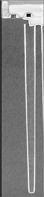
Figure 6.18: Deep trench DRAM bit cell.
A dynamic RAM, or DRAM for short, stores a bit in form of charge on a capacitor. Figure 6.19 shows the DRAM bit cell consisting of the capacitor and an nMOS transistor. If the capacitor is discharged to GND, we interpret the bit stored in the cell as logical 0. Otherwise, if the capacitor is charged to \(V_{DD},\) we interpret the stored bit as logical 1. The nMOS transistor controls the cell. If the wordline is 1, the nMOS transistor enables the cell by connecting the capacitor to the bitline. Otherwise, if the wordline is 0, the nMOS transistor is switched off, and disables the cell by disconnecting the capacitor from the bitline.

Figure 6.19: DRAM bit cell storing a 0 (left) and a 1 (right).
When reading the DRAM bit cell, the nMOS transistor connects the capacitor to the bitline. If the capacitor is discharged, we observe a zero voltage at the data output of the bitline. Otherwise, the charge of the capacitor diffuses onto the bitline, and we observe a logical 1 at the data output. Since the charge diffuses due to reading, we need to restore the bit cell after reading it. This is the reason why a DRAM is called dynamic RAM. Restoring the bit cell simply means writing the read value by driving it onto the bitline again, see Figure 6.16. The capacitor must be large enough so that a positive charge can be detected at the data output of the bitline. Figure 6.18 shows a deep trench capacitor, where a deep hole is drilled into a silicon wafer that is filled with metal. Since real capacitors leak, the charge stored on the capacitor must be restored periodically or the bit is lost.
The SRAM is a static RAM where the bit cell is stable because its state is continuously replenished by the power supply. An SRAM cell is essentially a bistable inverter pair. As shown in Figure 6.20, we control the inverter pair with two nMOS transistors and extend the memory array with a complemented bitline. Since each CMOS inverter requires two transistors, the bit cell as a whole consists of six transistors (6T). When the wordline is 0, the nMOS transistors disconnect the inverter pair from the bitlines. Otherwise, the bitlines are connected to the complemented and uncomplemented bit \(Q\) stored in the cell. We read the bit of the enabled cell at the data outputs of the bitlines. Writing a bit requires drivers at the data inputs of the bitlines that are stronger (larger) than the inverters of the cell, so as to overpower the inverter pair into the desired state.

Figure 6.20: 6T SRAM bit cell.
DRAM and SRAM memories are sequential circuits. However, neither memory design requires a clock signal for its operation. Therefore, DRAMs and SRAMs are asynchronous sequential circuits in principle. To operate within a synchronous design, memory arrays are wrapped into synchronous control logic to ensure that the read and write operations stabilize within a clock cycle. Figure 6.21 shows a black-box synchronous memory module. It has a clock input, a write-enable input WE, an \(n\)-bit address input, and an \(m\)-bit data input and \(m\)-bit data output.

Figure 6.21: Synchronous memory module.
The read operation of a synchronous memory module is considered a combinational operation, independent of the triggering clock edge. Reset the WE input to 0, apply the desired address \(A,\) and the associated data word appears at data output \(D_{out}\) after the propagation delay within one clock cycle. In contrast, the write operation is synchronized by the clock. Set the WE input to 1, apply the desired address \(A\) and data input \(D_{in},\) and the data is written into memory at the triggering positive clock edge.
The bus width of the address input specifies the number of rows, also called depth, of the memory array. Given \(n\) address wires, the \(n{:}2^n\) address decoder drives \(2^n\) wordlines, as shown in Figure 6.15, so that the depth of the memory array is \(2^n.\) The bus width of the data input and the data output is equal to the number of columns, also called width or word size, of the memory array. Thus, the memory array inside the synchronous memory module in Figure 6.21 has a width of \(m.\) The capacity of a memory is the number of bit cells, i.e. depth \(\times\) width bits. The memory array in Figure 6.15, for example, has 2 address bits, a depth of \(2^2 = 4,\) a width of 3, and a capacity of \(4 \times 3 = 12\) bits.
Logic in Memories
Memories serve not only their purpose as a storage medium but are also used as universal logic operators. Given a \(n\)-variable logic function, we use a \(2^n \times 1\) memory array with \(n\) address inputs and one data output as a lookup table to read the function values. We can configure a RAM to implement any logic function by storing one function value per row. Essentially, the memory stores the truth table of a given combinational function and we select the row by applying the desired input combination. Figure 6.22 shows a 2-input XOR function \(Y = A \oplus B,\) implemented by means of a \(4\times 1\) memory array.
A = 0 B = 0 Figure 6.22: 2-input XOR gate implemented with a \(4\times 1\) memory array.
Memories can implement multioutput functions by including one column per output. Thus, a multioutput function with \(m\) outputs can be realized with a memory array of width \(m.\) Since RAMs permit configuring any multioutput function that fits the depth and width of the memory array, RAMs serve as lookup tables in reconfigurable logic devices, including FPGAs.
Analyze the synchronous sequential NAND loop.

- Derive the next-state logic.
- Derive a state transition table.
- Derive a state transition diagram.
- Use a time table to analyze the transitions of input sequence \(A = \langle 0, 0, 1, 0, 0, 0, 1, 1, 1, 1 \rangle.\)
The sequential NAND loop has a register on the feedback path. The state of the present clock cycle is observable at register output \(Q.\) The next state is the value of the data input of the register, and is stored at the next positive clock edge. In the NAND loop, the next state equals output \(Y,\) and is a function of present state \(Q\) and input \(A\):
\[Y(A,Q) = \overline{A Q}\,.\]This function is the combinational next state logic of the circuit.
The state transition table is the truth table of the next state logic:
\(A\) \(Q\) \(Y\) 0 0 1 0 1 1 1 0 1 1 1 0 The state transition diagram is the graphical representation of the state transition table. It has one vertex per state, here \(Q \in \{ 0, 1 \},\) and one arc per transition. We annotate the arcs with input \(A\) and output \(Y,\) separated by a slash. Note that output \(Y\) is also the next state of the NAND loop.

The diagram shows that the NAND loop transitions from state \(Q=0\) to state \(Q=1\) regardless of input \(A.\) Thus, when the circuit transitions into state \(Q=0,\) it remains there for one clock cycle before returning to state \(Q=1.\) It remains in state \(Q=1\) while input \(A=0,\) and transitions to state \(Q=0\) when input \(A=1.\) If we hold input \(A\) at value 1, the circuit toggles between states 0 and 1 at every positive clock edge. This behavior resembles the oscillation in Exercise 6.1.
We use a time table to study the behavior of the NAND loop over time given input sequence \(A\) for ten clock cycles, \(0 \le t < 10\):
t 0 1 2 3 4 5 6 7 8 9 Q X 1 1 0 1 1 1 0 1 0 A 0 0 1 0 0 0 1 1 1 1 Y 1 1 0 1 1 1 0 1 0 1 We do not need to know initial state \(Q[0]\) during clock cycle \(t = 0\) to conclude that next state \(Y[0]=1\) if \(A=0.\) Therefore, we mark \(Q[0] = X\) as unspecified. While \(A=0,\) the circuit stays in state 1, and toggles between states 0 and 1 while \(A=1.\)
6.3. Finite State Machines
Finite state machines, or FSMs for short, are a subset of synchronous sequential circuits with a finite number of states. Although state machines with infinitely many states are of minor practical relevance, the distinction hints at the theoretical importance of FSMs as an abstract model for the study and design of sequential circuits.[1] In this section, we discuss FSMs and their use as a design methodology for synchronous sequential circuits.
6.3.1. Mealy and Moore Machines
Our study of synchronous circuits has revealed nuances in the behavior of such circuits. In particular, the multiplexer loop has an output which is a function of the input and the state, whereas the output of the binary counter is a function of the state only. Since the output of the multiplexer loop is a function of the input, the output may change during a clock cycle if the input changes. In contrast, the output of the binary counter remains stable during the clock cycle. We exploit this difference by tailoring the annotations in the state transition diagrams of Figure 6.9 and Figure 6.12 to their respective needs. In fact, these circuits examplify two distinct types of synchronous sequential circuits.
Machine Models
FSMs are generalizing models of synchronous sequential circuits. Figure 6.23 shows the Mealy machine model, named after George H. Mealy, and Figure 6.24 shows the Moore machine model, named after Edward F. Moore. Both machines have
- input bus \(I\) with \(m \ge 0\) signals \(I_0, I_1, \ldots, I_{m-1},\)
- output bus \(O\) with \(n \ge 0\) signals \(O_0, O_1, \ldots, O_{n-1},\)
- current state \(S\) stored in a \(k\)-bit state register with output signals \(S_0, S_1, \ldots, S_{k-1},\) \(k > 0,\) and capable of encoding up to \(2^k\) distinct states,
- next state \(S'\) with \(k\) signals \(S'_0, S'_1, \ldots, S'_{k-1},\)
- combinational next state logic \(\sigma,\) and
- combinational output logic \(\omega.\)
The next state logic of both Mealy and Moore machines is a combinational function \(\sigma: \mathcal{B}^{m+k}\rightarrow \mathcal{B}^k\) that computes next state \(S' = \sigma(S,I).\) The next state computation receives the present or current state \(S\) via the feedback loop. The loop includes the state register triggered by clock signal \(\phi,\) which qualifies both machines as synchronous sequential circuits.

Figure 6.23: Mealy machine model. Output \(O\) depends on state \(S\) and input \(I.\)
The essential difference between the two machine models is the combinational output logic \(\omega.\) For the Mealy machine, output function \(\omega: \mathcal{B}^{m+k} \rightarrow \mathcal{B}^n\) computes output \(O = \omega(S,I)\) as a function of current state \(S\) and input \(I.\) In contrast, the output function of the Moore machine \(\omega: \mathcal{B}^k \rightarrow \mathcal{B}^n\) computes output \(O = \omega(S)\) as a function of current state \(S\) only. The only difference in the circuit diagrams is that the Mealy machine connects input terminal \(I\) to combinational output logic \(\omega\) whereas the Moore machine does not. As a matter of convention for this chapter, we distinguish combinational and sequential logic in circuit diagrams by drawing black-box subcircuits of combinational logic as rectangles with round corners.

Figure 6.24: Moore machine model. Output \(O\) depends on state \(S\) only.
Machine Identification
It is not always immediately obvious which type of machine, Mealy or Moore, a synchronous sequential circuit implements. In fact, it may take several attempts of restructuring a circuit before it fits the structure of the Mealy machine in Figure 6.23 or the Moore machine in Figure 6.24. However, the distinguishing characteristic is usually straightfoward to check, i.e. whether the output is a function of the input or not. Consider the multiplexer loop in Figure 6.8, for example. Output \(Y\) is a function of state \(Q\) and inputs \(D\) and \(S.\) Therefore, the circuit is a Mealy machine. But, what is its next state logic \(\sigma\) and what its output logic \(\omega\)? Since the multiplexer output drives both output \(Y\) and the next state input of the D-flipflop, the circuit in Figure 6.8 does not have the structure of the Mealy machine in Figure 6.23. Nevertheless, duplicating the multiplexer, as shown in Figure 6.25, reveals that the multiplexer loop is an optimized version of a vanilla Mealy machine that reuses the next state logic as output logic or vice versa.

Figure 6.25: Multiplexer loop of Figure 6.8 (left) with duplicated multiplexer to match the Mealy machine model of Figure 6.23 (right).
As another example, consider the shift register in Figure 6.13. The outputs \(Y_0,\) \(Y_1,\) \(Y_2,\) and \(Y_3 = S_{out}\) are driven by the registers. Therefore, the outputs are a function of the current state but not a function of input \(S_{in}.\) We conclude that the circuit is a Moore machine. The topology of the circuit in Figure 6.13 is simpler than that of the equivalent vanilla Moore machine in Figure 6.26, where the next state logic \(\sigma\) and output logic \(\omega\) are identity functions.

Figure 6.26: Shift register of Figure 6.13 (left) and with alternative topology of a Moore machine, see Figure 6.24 (right).
Since Mealy and Moore machines differ in their output behavior only, we can often use either type to solve a given problem. However, if we wish to generate the output within the cycle of a particular state and input, then a Mealy machine is required. A Moore machine cannot change the output while in the particular state. Instead, in a Moore machine we must wait until the next triggering clock edge, where the machine assumes the next state as a function of the particular state and input, and can then produce the desired output. On the other hand, a Moore machine has a more robust timing behavior, because the consumer of the output can rely on the fact that the output is stable during the entire cloci cycle after the propagation delay of the output logic has elapsed follwing the triggering clock edge. This delay is independent of changes of the input of the machine.
Machine Transformations
Occasionally FSM designers perceive a Moore machine as more natural than a Mealy machine. If a particular type of machine is desired, such perceptions can be overcome because we may translate one machine type systematically into the other. Figure 6.27 shows the two graphical rules for translating state \(A\) from a Mealy type into a Moore type state transition diagram and vice versa. Recall that we associate the output in a Mealy diagram with the input and in a Moore machine with the state.

Figure 6.27: Rules for transforming a Mealy state diagram into a Moore state diagram and vice versa.
Rule 1 states that state \(A\) in Mealy machine can be translated into an equivalent state \(A\) in a Moore machine if all incoming transitions of the Mealy machine have the same output. In this case, we associate the output with state \(A\) of the Moore machine. Conversely, we translate state \(A\) of a Moore machine into a Mealy machine by associating output \(O\) of the Moore machine with all inputs in the Mealy machine. Rule 2 covers the case where the incoming arcs of state \(A\) in the Mealy machine have different outputs. In this case, we replicate Mealy state \(A\) in the Moore machine for each distinct output. Conversely, we transform the Moore machine into a Mealy machine by merging Moore states \(A_1\) and \(A_2\) into Mealy state \(A,\) and by associating the outputs of the Moore states with the inputs of the Mealy transitions.
Rule 2 is the reason why, in general, Mealy machines require fewer states than Moore machines to solve a given problem. Hence, a Mealy machine may be constructed with fewer D-flipflops than the equivalent Moore machine. Whether the reduction in state bits leads to an overall savings in logic, including the next state and output logic, depends on the particular implementation, and requires a direct comparison of alternative designs.
6.3.2. Synthesis of Finite State Machines
The FSM designer uses the tools for the analysis of synchronous circuits, in particular the state transition diagram and the state transition table, to specify a FSM for a given problem description, and to implement the FSM as a synchronous sequential circuit. FSM synthesis may be viewed as reversal of the analysis procedure. Although synthesis requires more creativity than analysis, the synthesis of FSMs is a relatively systematic process.
The design methodology for an FSM can be summarized as a 6-step recipe:
- Identify inputs and outputs.
- Design a state transition diagram.
- Select a state encoding.
- Derive the state transition table.
- Minimize the next state and output logic.
- Synthesize the circuit.
Most of a designer’s creativity flows into step 2, where a problem description, typically provided as an informal statement, is formalized by means of a state transition diagram either of Mealy type or of Moore type. The other five steps are comparatively straightforward applications of established techniques.

Before we illustrate the FSM design methodology by means of several examples, let us clarify the role of the state register as the central element of every FSM. The state register holds the current state \(S,\) which we may observe at its output \(Q.\) State \(S\) remains stable for the entire clock cycle between triggering clock edges. Next state \(S'\) is stored at the next triggering clock edge. The next state logic computes \(S'\) as a function of the inputs \(I\) and current state \(S.\) Next state \(S'\) must be stable before the next triggering clock edge so that the state register can store the next state reliably. In Moore machines, the state register decouples the outputs from the inputs. Since the outputs are a function of current state \(S\) only, the inputs affect the outputs of the next state indirectly. In contrast, in a Mealy machine, the inputs bypass the state register so that the outputs react to changes at the inputs within the current clock cycle.
Serial Adder
We wish to design a serial version of a ripple carry adder. Assume that the binary summands appear one bit per clock cycle at inputs \(A\) and \(B,\) least significant bits first. The adder shall output the sum bits one per clock cycle, lsb first.

Following the design recipe, we find that step 1 is trivial whereas step 2 requires some thought. Recall that bit position \(i\) might generate a carry into position \(i+1.\) Since the summands appear at the inputs lsb first, imagine the lsb‘s appear in cycle 0, the bits of next position 1 in cycle 1, and so on. Thus, the bits of the summands in position \(i\) are available in cycle \(i,\) and we need to make the carry out of position \(i\) available as carry input during cycle \(i+1.\) We conclude that we need a 1-bit register that stores the carry-out at the next triggering clock edge, which separates current cycle \(i\) and next cycle \(i+1\) in time. The output of the register is the carry-in during cycle \(i+1.\) Since bit position \(i\) generates a carry or not, a 1-bit register suffices to distinguish these two states. Therefore, we decide to design the FSM with a 1-bit state register. Furthermore, we decide to design a Mealy machine.
We develop the state transition diagram of the Mealy machine, starting with two state vertices for state S0, meaning the carry-in is 0, and state S1 to represent a carry-in equal to 1 during the current clock cycle. Figure 6.28(a) shows the two state vertices. Next, we consider the state transitions. Since the current state represents the carry-in, the next state represents the carry out. Thus, our next state logic must implement the carry-out function of a full adder. The carry-out, i.e. the next state, is a combinational function that depends on the two inputs \(A\) and \(B\) and the carry-in, i.e. the current state \(S.\)

Figure 6.28: Design of state transition diagram for serial adder.
Recall that the carry-out of a full adder is 1 if two or three inputs are 1, and otherwise the carry-out is 0. First, we consider the outgoing transitions of state S0, see Figure 6.28(b). The only input combination that can generate a carry-out of 1 is \(A = B = 1.\) We draw an arc from S0 to S1, and annotate it with input combination \((A,B)=11.\) The remaining three input combinations do not generate a carry out. Therefore, we draw a looping arc at state S0, and annotate it with the three remaining input combinations. The outgoing transitions of state S1 are shown in Figure 6.28(c). With a carry-in equal to 1, the only input combination that causes the carry-out to be 0 is \(A = B = 0.\) We draw an arc from S1 to S0 for input combination \((A,B) = 00.\) The other three input combinations cause a carry-out of 1, represented by the loop pointing from S1 to S1. In Figure 6.28(d), we add the outputs to each input combination. The output of the serial adder is the sum bit. If the carry-in is 0, i.e. in state S0, the sum is 1 if exactly one of the inputs \(A\) or \(B\) is 1, otherwise the sum is 0. In state S1, representing a carry-in of 1, the sum is 1 if inputs \(A\) and \(B\) are equal. We also mark state S0 with another circle, indicating that S0 is the start state of the Mealy machine, because initially the carry into lsb position 0 should be 0.
Step 3 of the FSM recipe requires selecting a state encoding. We choose the natural encoding suggested by our design, \(S0 = 0\) and \(S1 = 1,\) because the state register should store the value of the carry. Using the opposite encoding is possible, but would be rather confusing. Next, we derive the state transition table according to step 4 of the FSM recipe. It shouldn’t come as a surprise that converting the state transition diagram of Figure 6.28(d) into a state transition table yields the truth table for the carry-out of a full adder, where the current state is the carry-in:
state A B next state Sum 0 0 0 0 0 0 0 1 0 1 0 1 0 0 1 0 1 1 1 0 1 0 0 0 1 1 0 1 1 0 1 1 0 1 0 1 1 1 1 1
We have included the Sum output of the serial adder in the state transition table, because it adds just one more column to the truth table. Since the output of a Mealy machine is a function of the current state and the inputs, needed for the next state as well, this is faster and less error-prone than compiling a separate truth table for the output function. Note that the translation of the state transition diagram into the state transition table is a straightforward transliteration of the directed graph into truth table format. No knowledge specific to the purpose of our adder design is required, except the state encoding.
Step 5 of the FSM recipe asks us to minimize the next state and output logic. To that end, we apply the techniques developed for combinational logic design, for example K-maps. The K-maps for the next state \(S'\) and the Sum output

yield the well-known SOP expressions of the majority and odd-parity functions
Without further logic optimizations or technology mapping, we complete step 6 of the FSM recipe, and synthesize a circuit diagram for the serial adder using two-level combinational logic. Figure 6.29 shows the resulting Mealy machine in the topological form of Figure 6.23. The next state logic \(\sigma\) is the majority function and output logic \(\omega\) is a 3-variable XOR function.

Figure 6.29: Mealy machine for serial adder.
Figure 6.29 completes the FSM design of the serial adder. Note that the serial adder consists of the combinational logic of one full adder plus one register. Compared to a ripple carry adder, which requires \(n\) full adders to add two \(n\)-bit summands, our serial adder FSM requires only one full adder, independent of \(n.\) However, our serial adder FSM requires \(n\) clock cycles to produce all sum bits. This is a typical example for the trade-off between space and time in digital logic.
Now that we have a Mealy machine, we have two options to design a Moore machine for the serial adder. Option 1 is to start from scratch, working ourselves through the six steps of the FSM recipe. However, step 2 of the recipe requires more creativity for a Moore machine than for the Mealy machine. This becomes clear after working through Option 2, deriving the Moore machine from the Mealy machine using machine transformations. The state transition diagram of the Mealy machine in Figure 6.28(d) shows four incoming transitions for each state with different outputs, 0 or 1. Therefore, we apply Rule 2 and split each Mealy state into two Moore states, as shown in Figure 6.30. Moore state \(S0_0\) represents a carry-in of 0 with sum output 0 and Moore state \(S0_1\) represents a carry-in of 0 with sum output 1. Analogously, Moore states \(S1_0\) and \(S1_1\) represent a carry-in of 1 with the corresponding outputs.

Figure 6.30: State transition diagram of Moore machine for serial adder.
The state transition diagram of the Moore machine in Figure 6.30 is significantly more complex than the corresponding diagram of the Mealy machine. This is, of course, why we present the design of the Mealy machine for the serial adder to begin with. We leave it as an exercise to complete the design of the Moore FSM.
Pattern Recognizer
We receive a periodic binary signal and wish to recognize patterns of two consecutive 1’s. To solve this problem, we follow the FSM design recipe.

At the first glance, the problem description appears to be rather vague. However, step 1 of the recipe gives us a chance to tie up loose ends by defining the inputs and outputs of our pattern recognizer machine. The binary signal constitutes a 1-bit input; call it \(A.\) Since the binary signal is periodic, we assume a clock signal \(\phi\) with the period of input \(A.\) To indicate recognition of two consecutive 1’s in input \(A,\) we attach a 1-bit output, say \(Y,\) to the machine. Our goal is to set output \(Y\) to 1 after recognizing two consecutive 1’s in \(A\) and to 0 otherwise. The block diagram on the right summarizes our findings.
Following step 2 of the design recipe, we model the problem as a state transition diagram. With little information in the problem description to go on, our best bet is to examine the sampling behavior of the input signal with a concrete example. As shown in Figure 6.31, we assume that clock \(\phi\) and input \(A\) have the same period. Furthermore, to facilitate reliable sampling, input signal \(A\) must be stable before and at the positive clock edge. As shown in the waveform diagram, we assume that signal \(A\) changes shortly after the positive clock edge. Thus, \(A\) is stable during most of the clock cycle and, in particular, at the triggering clock edge at the end of the cycle. This timing behavior gives our machine enough slack to compute the next state during the clock cycle, and store the next state at the end of the cycle. Under these assumptions, we count time in the waveform diagram in multiples of clock cycles.

Figure 6.31: Waveform diagram of Moore type pattern recognizer.
To simplify the problem even further, we ignore the details of the timing behavior, and use abstract binary sequences for the input and output signals of the machine. The input sequence in Figure 6.31 is
In the following, we refer to element \(i\) of sequence \(A\) as \(A[i],\) and interpret \(A[i]\) as the Boolean value of input signal \(A\) during cycle \(i.\) For example, \(A[0] = 0\) and \(A[2] = 1.\)
Next, we develop the desired output signal for input sequence \(A.\) Assume output \(Y\) is initially 0, until we have seen the first pair of inputs \(A[0] = 0\) in cycle 0 and \(A[1] = 0\) in cycle 1. Since two consecutive 0’s differ from the 11-pattern we are looking for, we set the output to 0. Since we need to inspect the inputs during cycles 0 and 1, it seems natural to assign 0 to output \(Y\) during cycle 2 after receiving two input bits. Thus, we pursue a timing behavior where the machine inspects the first input bit \(A[t]\) during cycle \(t,\) the second input bit \(A[t+1]\) during cycle \(t+1,\) and asserts the corresponding output \(Y[t+2]\) during cycle \(t+2.\) In Figure 6.31, the first pair of consecutive 1’s is \(A[2]=1\) and \(A[3]=1,\) so that cycle 4 is the first cycle where we set \(Y[4]=1.\) During cycle 5 we set \(Y[5]=0,\) because \(A[3] =1\) and \(A[4]=0.\) The second pair of consecutive 1’s appears in cycles 8 and 9, \(A[8]=1\) and \(A[9]=1.\) Therefore, we set \(Y[10]=1.\) Cycle 9 presents a notable case, because \(A[9]=1\) and \(A[10]=1.\) Hence, we set \(Y[11]=1.\) This case is notable, because input \(A[9]=1\) belongs to two overlapping pairs of 11-patterns. We interpret our problem description to recognize 11-patterns as recognizing every 11-pattern, and include overlapping patterns. As a result our pattern recognizer should produce the output sequence
for input sequence \(A.\)
The sequence abstraction is crucial for the design of a finite state machine. First, however, we have to decide on the type of the machine, Mealy or Moore machine. Our earlier decision to assign the output during the cycle after inspecting two consecutive input bits implies a Moore machine. The waveform diagram in Figure 6.31 clarifies this implication. Consider cycle 4, where output \(Y[4]=1\) in response to recognizing 11-pattern \(A[2] = A[3] = 1.\) Output \(Y\) should be independent of input \(A,\) or \(Y\) might switch to 0 during cycle 4 when \(A\) switches from 1 to 0. In a Moore machine, output \(Y\) is independent of the input and, therefore, switches at the triggering clock edges only, as indicated by the arrows in Figure 6.31.
We are ready to design the state transition diagram for a Moore type pattern recognizer. Since the number of required states is not immediately obvious, we develop the states incrementally. We begin with start state S0, where we wait for the first 1 to appear in input \(A.\) When the first 1 occurs, we transition to a new state S1. Otherwise, we stay in state S0 and output \(Y=0.\) Figure 6.32(a) shows start state S0 and its two outgoing transitions. Next, consider state S1. We transition into S1 after observing one 1 on input \(A.\) Since we have not observed two 1’s, we output \(Y=0.\) If we observe input 0 while in S1, we return to S0, and wait for the next 1 to appear. Otherwise, if we observe input 1, we transition to new state S2, see Figure 6.32(b). In state S2, we have received two consecutive 1’s in the two preceding cycles. Therefore, we output \(Y=1.\) The transitions out of state S2 are shown in Figure 6.32(c). If we observe input 1, we encounter the case of overlapping 11-patterns. We remain in state S2 and output \(Y=1.\) Otherwise, if input \(A=0,\) we return to state S0 and wait for the next 1 to appear in the input. This completes the state transition diagram.

Figure 6.32: Design of state transition diagram for Moore type pattern recognizer.
We continue with step 3 of the design recipe, and select a state encoding. The Moore machine in Figure 6.32(c) has three states. Thus, we need at least \(\lceil \lg 3\rceil = 2\) bits to encode three states. We choose a binary encoding of the state number:
state binary encoding S0 00 S1 01 S2 10
The binary encoding seems natural, but is not necessarily the best choice. Other choices may reduce the cost of the next state and output logic. However, the binary state representation minimizes the width of the state register. For our Moore machine, we need a 2-bit state register with binary state \(S = S_1 S_0.\)
Given the state encoding, we can develop the state transition table according to step 4 of the design recipe. The table defines the state \(S' = S_1' S_0'\) as a function of the current state \(S = S_1 S_0\) and input \(A.\) For clarity, we also include columns for the corresponding state names used in the state transition diagram of Figure 6.32(c).
\(S\) \(S_1\) \(S_0\) \(A\) \(S'\) \(S_1'\) \(S_0'\) S0 0 0 0 S0 0 0 S0 0 0 1 S1 0 1 S1 0 1 0 S0 0 0 S1 0 1 1 S2 1 0 S2 1 0 0 S0 0 0 S2 1 0 1 S2 1 0
The state transition table is a truth table that specifies the combinational next state logic. More succinctly, the next state logic is a multioutput function \(S' = \sigma(S, A)\) where \(S_1'\) and \(S_0'\) are Boolean functions in three variables, \(S_1,\) \(S_0,\) and \(A.\)
Furthermore, we compile a truth table for the output logic. Output \(Y\) of the Moore machine is a function of the current state \(S = S_1 S_0.\) The state transition diagram in Figure 6.32(c), specifies in each state vertex the associated output, which we summarize in a separate truth table.
\(S\) \(S_1\) \(S_0\) \(Y\) S0 0 0 0 S1 0 1 0 S2 1 0 1
Following step 5 of the design recipe, we minimize the next state and output logic. We use K-maps for the incompletely specified functions

to derive the minimal SOP expressions
Last but not least, we obtain the circuit diagram in Figure 6.33, which realizes step 6 of the design recipe. The output logic is the trivial identity function. To enter start state S0, we assume that the register has a separate reset input that enables us to reset all D-flipflops.

Figure 6.33: Pattern recognizer as Moore machine.
Now that we have a complete design for the pattern recognizer as a Moore machine, we amortize our intellectual investment by designing a Mealy machine for direct comparison. We restart the design process at step 2 of the recipe. Figure 6.34 shows the waveform diagram with the same input signal as in Figure 6.31, assuming that output \(Y\) depends not only on the state but also on input \(A.\) We exploit the combinational dependence on input \(A\) to redefine the timing behavior of output \(Y,\) such that \(Y=1\) during the clock cycle when the second 1 appears on input \(A.\) More precisely, if \(A[t] = 1\) during cycle \(t\) and \(A[t+1] = 1\) during cycle \(t+1,\) then we can set \(Y[t+1]=1\) in a Mealy machine, which is one cycle earlier than in the Moore machine.

Figure 6.34: Waveform diagram of Mealy type pattern recognizer.
Consider the first occurance of two consecutive 1’s in cycles 2 and 3. The Mealy machine sets output \(Y\) to 1 during cycle 3 already. Note that output \(Y\) will remain 1 at the beginning of cycle 4 until \(A\) changes from 1 to 0. Indeed, the timing behavior of output \(Y\) of the Mealy machine is not as clean as that of the Moore machine. The output may even exhibit glitches as at the beginning of cycle 6. However, if we sample output \(Y\) toward the end of the cycle, then the behavior is as expected: we observe \(Y=1\) at the positive clock edges at the end of cycle 3, cycle 9, and cycle 10.
The state transition diagram of the Mealy machine requires only two states. State S0 is the start state, which waits for the first 1 to appear on input \(A.\) When \(A=1,\) we transition to state S1, and output \(Y=0.\) If \(A=1\) in state S1, the 1 input must have been preceded by another 1, so we output \(Y=1\) and remain in state S1. If input \(A = 0\) in state S0 or S1, the machine outputs \(Y=0\) and transitions to next state S0. The Mealy machine saves one state compared to the Moore machine.

Figure 6.35: State transition diagram for Mealy type pattern recognizer.
The remaining steps of the design recipe involve straightforward design work. Since the Mealy machine has two states, we need a 1-bit register to store \(S=0\) representing state S0 and \(S=1\) for state S1. We translate the state transition diagram in Figure 6.35 into the combined truth table for the next state logic and output logic:
\(S\) \(A\) \(S'\) \(Y\) 0 0 0 0 0 1 1 0 1 0 0 0 1 1 1 1
We can spot the minimal Boolean expressions in the truth table without the aid of K-maps: next state \(S' = A\) and output \(Y = A \cdot S.\) The resulting circuit diagram of the Mealy machine is shown in Figure 6.36. The machine is a degenerate Mealy machine without a feedback loop.

Figure 6.36: Pattern recognizer as Mealy machine.
Comparison with the Moore machine in Figure 6.33 shows that the Mealy machine needs one D-flipflop rather than two and only one gate rather than four. These hardware savings come at the expense of a noisy timing behavior. If the clean timing behavior of the Moore machine output is desired, we can have it albeit at increased hardware cost.
Traffic Light
Perhaps the seminal application of finite state machines is the traffic light controller. The animation in Figure 6.37 shows the baroque Austrian style, which ends the green phase in a flashy trill.
Figure 6.37: Austrian traffic light animation.
Designing a controller FSM for the traffic light requires determining a suitable clock period. A simple, natural choice is the shortest duration that any light is switched on or off. Assume that the blinking green light at the end of the green phase determines the clock period \(T,\) and all other phases last a multiple of \(T\):
phase duration red \(13\,T\) red-yellow \(4\,T\) green \(5\,T\) green blinking \(1\,T \times 4\) yellow \(4\,T\)

Given this problem description, we design an Austrian traffic light controller follwing the FSM recipe. First, step 1, we define the inputs and outputs. Other than the clock signal, our rudimentary controller receives no data inputs. Standard traffic lights consist of three colored lights, red, yellow, and green. The controller switches each of the three lights on or off. Therefore, we attach three 1-bit outputs, \(R,\) \(Y,\) and \(G.\) If the output is 1, the associated light shall be switched on and otherwise off.
Next, step 2, we design a state transition diagram. Since the controller has no input signals, we do not have a choice but construct a Moore machine. We introduce one state per clock cycle, for a total of 34 states. The green blinking phase consists of four times two cycles, one cycle green off plus one cycle green on. Figure 6.38 shows the Moore type state transition diagram. If an output equals 1, we include the associated output letter in the state vertex. Absence of the output letter means the output shall be 0.

Figure 6.38: State transition diagram for traffic light controller.
To encode 34 states, step 3, we need \(\lceil \lg 34\rceil = 6\) bits if we use a binary state encoding \(S = S_5 S_4 S_3 S_2 S_1 S_0.\) The number of states is large enough to get us into trouble with the minimization of the next state and output logic. K-maps for six variables do exist, but algorithmic minimization methods may be preferable in this case. Rather than following the FSM recipe, we develop a more creative solution to turn the state transition diagram into a synchronous circuit. We note that the state sequence equals that of a binary counter modulo 34. Thus, rather than deriving minimal expressions for each of the six next state functions, we extend the binary counter in Figure 6.11 to generate the desired state sequence. We transition from state S33 to S0 by asserting the reset signal if the current state is equal to \(33_{10} = 100001_2,\) or in terms of Boolean algebra:
Minimizing the output functions individually, we find the SOP expressions as functions of the current state:
The resulting circuit diagram of the traffic controller is shown in Figure 6.39, with the output logic hidden in a black box,

Figure 6.39: Circuit diagram of traffic light controller.
This example illustrates the design problem with monolithic finite state machines. If the number of states becomes too large, steps 4-6 of the FSM design recipe become unmanageable. At this point, we may compose the machine out of smaller machines. We discuss the composition of FSMs as an alternative design methodology below.
A divide-by-2 frequency divider asserts output \(Y\) for one clock cycle out of 2:

- Design a synchronous divide-by-2 frequency divider.
- Verify your circuit by deriving its state transition diagram.
The waveform of the divide-by-2 frequency divider suggests that output \(Y\) toggles between 0 and 1 at every positive clock edge. Thus, we may use a register to store present state \(Q,\) and use an inverter to toggle next state \(Q' = \overline{Q}.\) The sequential circuit below connects output \(Y\) to the output of the inverter, so that \(Y = Q'.\)

The problem is simple enough to ignore the FSM recipe and derive the frequency divider machine in an ad hoc fashion.
We analyze our machine design by deriving its state transition diagram. Since the state register stores one of two states \(Q \in \{ 0, 1\},\) the transition diagram has two vertices. The machine has no inputs other than clock signal \(\phi.\) Instead, whenever the machine is in state \(Q = 0\) it transitions to state \(Q = 1\) and vice versa. Therefore, we annotate the arcs with the corresponding output \(Y=Q'\) only.

The state transition diagram enables us to grasp the behavior of the frequency divider easily. The machine toggles between states 0 and 1, and outputs 1 in state 0 and 0 in state 1. This is the expected behavior given the waveform above. In fact, we could have connected output \(Y\) to the output of the register rather than the output of the inverter, so that \(Y = Q.\) The behavior observed at output \(Y\) would be the same as for \(Y=Q',\) if we ignore the startup behavior of the machine. The only change in the state transition diagram would be complementing the outputs annotated at the arcs.
A divide-by-3 frequency divider asserts output \(Y\) for one clock cycle out of 3.

Design a state machine for the frequency divider following the FSM recipe:
- Identify inputs and outputs.
- Design a state transition diagram.
- Select a state encoding.
- Derive the state transition table.
- Minimize the next state and output logic.
- Synthesize the circuit, and determine the cost of the logic.
Given the waveform diagram, the frequency divider needs no input other than clock signal \(\phi,\) and one output signal \(Y.\)
The creative part of the design process consists of identifying the states for the state transition diagram. The divide-by-3 frequency divider exhibits periodic behavior with a period of 3 clock cycles. We set output \(Y=1\) during one of the 3 cycles and \(Y=0\) during the other two cycles of one period. Therefore, we introduce three states, \(S0,\) \(S1,\) and \(S2,\) corresponding to each of the three clock cycles:

We choose state \(S0\) to set output \(Y=1.\) This decision is arbitrary in the sense that the observer of output \(Y\) cannot distinguish the particular choice of the state unless the startup behavior of the machine is relevant. The states transition at every positive clock edge, so that each state is visited for exactly one clock cycle, and the output transitions accordingly. Since we associate an output with each state, our state transition diagram models a Moore machine.
To encode 3 states we need at least \(\lceil \lg 3\rceil = 2\) bits. We choose the natural binary encoding where \(S = S_1 S_0\) is an unsigned binary number:
state \(S_1\) \(S_0\) \(S0\) 0 0 \(S1\) 0 1 \(S2\) 1 0 Given the state encoding, we derive the state transition table by transliterating the state transition diagram. For each current state \(S,\) we include the next state \(S'\) and output \(Y\):
\(S_1\) \(S_0\) \(S'_1\) \(S'_0\) \(Y\) 0 0 0 1 1 0 1 1 0 0 1 0 0 0 0 This table specifies next state functions \(S'_1(S_1, S_0)\) and \(S'_0(S_1, S_0)\) and output function \(Y(S_1,S_0).\) These functions are incompletely specified, because the state transition table omits state \(S = 11_2.\)
We minimize the next state and output logic using K-map minimization for incompletely specified functions:

We find minimal covers \(S'_1 = S_0,\) \(S'_0 = \overline{S}_1\,\overline{S}_0,\) and \(Y = \overline{S}_1\,\overline{S}_0.\) Note that \(Y = S'_0,\) which is obvious because the columns in the state transition table are identical. Thus, we could have saved the minimization of \(Y.\)
We synthesize the frequency divider circuit at the gate level. The schematic includes a 2-bit state register, and the minimized next state logic and output logic using NOR technology:

The cost of the combinational logic of the frequency divider is the cost of two 2-input NOR gates for a total of \(\mathcal{C} = 4.\) The cost of the machine is the cost of the logic plus two 1-bit registers.
Redesign the divide-by-3 frequency divider of Exercise 6.4 with a one-hot state encoding.
Follow the FSM recipe:
- Identify inputs and outputs.
- Design a state transition diagram.
- Use a one-hot state encoding.
- Derive the state transition table.
- Minimize the next state and output logic.
- Synthesize the circuit, and determine the cost of the logic.
We redesign the divide-by-3 frequency divider of Exercise 6.4. This exercise requests a one-hot state encoding. Steps (1) and (2) of the FSM recipe remain unaffected by the state encoding. Therefore, we reuse the state transition diagram of step (2) in Exercise 6.4, and continue with step (3) of the FSM recipe.
A one-hot encoding of three states \(S0,\) \(S1,\) and \(S2,\) sets one bit out of three to 1. Therefore, our one-hot code words consist of three bits, \(S = S_2 S_1 S_0,\) such that:
state \(S_2\) \(S_1\) \(S_0\) S0 0 0 1 S1 0 1 0 S2 1 0 0 Given the one-hot state encoding, we derive the state transition table by transliterating the state transition diagram of Exercise 6.4 into a truth table:
\(S_2\) \(S_1\) \(S_0\) \(S'_2\) \(S'_1\) \(S'_0\) \(Y\) 0 0 1 0 1 0 1 0 1 0 1 0 0 0 1 0 0 0 0 1 0 The state transition table specifies four incomplete Boolean functions in three variables. We minimize these functions using K-map minimization:

We find the minimal covers \(S'_2 = S_1,\) \(S'_1 = S_0,\) \(S'_0 = S_2,\) and \(Y = S_0 (= S'_1).\)
The synthesized circuit requires a 3-bit register and no logic gates:

The cost of the combinational logic is \(\mathcal{C} = 0.\) Compared to the binary encoding in Exercise 6.4, the one-hot encoding saves the logic cost entirely at the expense of one additional 1-bit register. Note that the one-hot frequency divider is a cyclically wired shift register.
Given a bit-serial input stream, design an odd parity checker that asserts its output when the input stream contains an odd number of 1’s.

Follow the FSM recipe:
- Identify inputs and outputs.
- Design a state transition diagram.
- Select a state encoding.
- Derive the state transition table.
- Minimize the next state and output logic.
- Synthesize the circuit.
The black-box diagram of the parity checker shows one input \(A\) and one output \(Y.\) We assume that the clock signal is supplied implicitly.
We design a state transition diagram for the odd parity checker with bit-serial input \(A\) and output \(Y.\) The specification requires that output \(Y\) is 1 when the number of 1’s in the input stream is odd. Before formalizing the specification, we clarify several details. To observe the number of 1’s in the input bit stream, we need to specify the start of the observation. Thus, we introduce clock cycle \(t,\) and let \(t = 0\) be the start cycle. Assuming our machine inspects input \(A[t-1]\) during cycle \(t-1,\) we set \(Y[t] = 1\) if the number of 1’s in sequence \(A[0{:}t-1] = \langle A[0], A[1], \ldots, A[t-1]\rangle\) is odd. A time table illustrates our design:
t 0 1 2 3 4 5 6 7 8 9 A 0 1 0 1 1 1 1 0 0 0 Y 0 0 1 1 0 1 0 1 1 1 During start cycle \(t=0,\) we set output \(Y=0\) indicating that no 1’s have been detected before the start cycle. Note that zero is an even number. The machine inspects input \(A[0] = 0,\) and computes the next output \(Y[1]=0,\) because the number of 1’s in sequence \(A[0{:}0] = A[0]\) is zero. During cycle \(t=1,\) the machine outputs \(Y[1]=0,\) and inspects input \(A[1]=1.\) Since the number of 1’s in sequence \(A[0{:}1] = \langle 0, 1\rangle\) is 1, i.e. an odd number, the next output is \(Y[2]=1.\) The remaining entries in the time table are derived analogously.
Next, we formalize our parity checker by designing the state transition diagram. The machine has two states \(Q \in \{ \text{even}, \text{odd}\}\) indicating whether the current number of 1’s in input sequence \(A\) is even or odd. If current state \(Q\) is even and input \(A=0,\) we remain in state even. Otherwise, if \(A=1,\) we transition into next state \(Q' = \text{odd.}\) If current state \(Q = \text{odd}\) and input \(A=0,\) we remain in state odd, and if \(A=1,\) we transition into next state even. The state transition diagram below captures these arguments in form of a graph:

We associate output \(Y\) with the states, keeping in mind that the state during clock cycle \(t\) and associated output \(Y[t]\) reflect the parity of the number of 1’s in input sequence \(A[0,t-1].\) Thus, our design is a Moore machine. We handle the remaining steps of the FSM recipe in a systematic fashion.
The state transition diagram suggests the state encoding:
state \(S\) even 0 odd 1 This encoding is convenient, and likely to produce a low-cost circuit, because output \(Y=S.\)
The state transition table specifies next state \(S'\) and output \(Y\) as functions of current state \(S\) and input \(A.\) We generate the table by straightforward transliteration of the state transition diagram and the chosen state encoding:
\(S\) \(A\) \(S'\) \(Y\) 0 0 0 0 0 1 1 0 1 0 1 1 1 1 0 1 We recognize Boolean functions \(S'\) and \(Y\) in the state transition table as \(S' = A \oplus S\) and \(Y = S.\)
The synthesized gate-level circuit for the odd parity checker is:

Note that output \(Y\) is not a function of input \(A\) but is a function of state \(S\) only. Thus, our parity checker is a Moore machine, indeed.
Consider a pattern recognizer for bit pattern 011.
- Design the state transition diagram of a Mealy machine.
- Design the state transition diagram of a Moore machine.
A pattern recognizer has input \(A\) and output \(Y.\) We set output \(Y = 1\) for one clock cycle if pattern 011 appears on input \(A.\)
A Mealy machine can respond to changes at its inputs within the current clock cycle, because the output is a function of the current state and the inputs. Therefore, we design the state transition diagram such that output \(Y\) is associated with the transition arcs. First, we study a concrete input sequence by means of a time table, however:
t 0 1 2 3 4 5 6 7 8 9 10 11 12 13 14 15 A 0 0 1 0 1 1 0 1 1 1 1 0 1 1 0 0 Y 0 0 0 0 0 1 0 0 1 0 0 0 0 1 0 0 Observe that pattern 011 appears at input sequence \(A\) during cycle interval \(3 \le t \le 5,\) interval \(6 \le t \le 8,\) and \(11 \le t \le 13.\) In a Mealy machine, we set output \(Y = 1\) during the cycle when the last 1 of the pattern appears, i.e. during cycles 5, 8, and 13. During all other cycles, we set output \(Y=0,\) as shown in the time table.
A Mealy machine needs three states to recognize pattern 011. State \(S0\) is the start state, were the machine waits until the first 0 appears at input \(A.\) Then, the machine transitions into state \(S1.\) If input \(A=1\) in state \(S1,\) the machine transitions into state \(S2.\) If input \(A=1\) in state \(S2,\) the machine recognizes pattern 011, and transitions back to start state \(S0.\) We include arcs from \(S0\) to \(S1\) for \(A/Y = 0/0,\) from \(S1\) to \(S2\) for \(A/Y = 1/0,\) and from \(S2\) to \(S0\) for \(A/Y = 1/1.\)

To complete the state transition diagram, we observe that each state must have two outgoing arcs, one for input \(A=0,\) and the other for \(A=1.\) Thus, we inspect each state and attach the outgoing arcs not discussed above. We need an arc from state \(S0\) to itself for \(A/Y = 1/0,\) because we wait in \(S0\) while input \(A=1\) until the first 0 appears. State \(S1\) waits until a 1 appears at the input. Thus, we need an arc from state \(S1\) to itself for \(A/Y = 0/0.\) If input \(A=0\) in state \(S2,\) the input pattern is 010, which differs from pattern 011. The last 0 may be the first 0 of pattern 011, however. Therefore, we need an arc from state \(S2\) to state \(S1\) for \(A/Y = 0/0.\)
A Moore machine computes its output as a function of the current state only. Therefore, a Moore machine responds to an input in the next clock cycle at earliest. The state transition diagram of a Moore machine associates the output with the state vertices. Before, designing the state transition diagram, we revisit the concrete example of subproblem (a), with output \(Y\) specified as expected for a Moore machine:
t 0 1 2 3 4 5 6 7 8 9 10 11 12 13 14 15 A 0 0 1 0 1 1 0 1 1 1 1 0 1 1 0 0 Y 0 0 0 0 0 0 1 0 0 1 0 0 0 0 1 0 Compared to the Mealy machine, we set output \(Y=1\) during the clock cycle after receiving the third bit of pattern 011, i.e. during clock cycles 6, 9, and 14. The Moore machine needs four states to recognize pattern 011. State \(S0\) is the start state. If input \(A=0,\) the machine transitions to state \(S1,\) from there to state \(S2\) if \(A=1,\) and to state \(S3\) if \(A=1\) again. In state \(S3,\) the machine signals that it recognizes pattern 011 by setting output \(Y=1.\) In the other states, output \(Y=0.\)

We complete the state diagram by visiting each state, and attaching the missing outgoing arcs. Since the machine has one input, each state vertex must have two outgoing arcs one for input \(A=0\) and the other for \(A=1,\) as in the Mealy machine. If input \(A=1\) in start state \(S0,\) we wait for the first 0. Thus, we need an arc from \(S0\) to itself for \(A=1.\) In state \(S1,\) we wait for one or more 0’s in the input. Thus, for input \(A=0\) we need an arc from \(S1\) to itself. In state \(S2,\) we have seen pattern prefix 01. If the input is \(A=0,\) this 0 may be the first 0 of pattern 011. Therefore, we include an arc from \(S2\) to \(S1\) for \(A=0.\) In state \(S3,\) we recognize pattern 011. If input \(A=0,\) this 0 may be the first 0 of pattern 011, and we include an arc from \(S3\) to \(S1.\) On the other hand, input \(A=1\) does not start pattern 011, and we include an arc to start state \(S0\) to wait for the next 0 again.
We conclude that the Moore machine requires one more state than the Mealy machine and the output responds one clock cycle later. We note that the synthesized circuit for the Moore machine is often more costly than the Mealy machine. In contrast the timing behavior of output \(Y\) of the Moore machine is less sensitive to the timing behavior of input \(A\) than the Mealy machine.
6.4. Composition of Finite State Machines
The 6-step design recipe for finite state machines represents a methodology which produces monolithic machines with a potentially large number of states. The traffic light controller is an example of a monolithic FSM design with 34 states. Larger FSMs with hundreds or even thousands of states are by no means uncommon in real-world applications. An alternative design methodology is the composition of larger FSMs from smaller FSMs with combinational glue logic. Given a large monolithic FSM, we may decompose or factor the machine into multiple smaller machines. In this section, we demonstrate the opposite design process. Rather than decomposing a given monolithic FSM, we start with a clean slate and demonstrate how to design a larger FSM by composing multiple smaller FSMs.
6.4.1. Primitive State Machines
We introduce several primitive state machines that serve as building blocks for larger state machines. We assume that all primitive state machines have a clock input and a reset input, without drawing them explicitly in our circuit diagrams. All clock inputs shall be driven by the same clock signal \(\phi\) so that the resulting state machine is a synchronous circuit. Similarly, all reset inputs shall be driven by the same reset signal, used to reset all D-flipflops to 0, for example to guarantee a well-defined start state.
Delay Element
The simplest primitive state machine is the delay element, which resembles a 1-bit shift register. The symbol of the delay element on the left in Figure 6.40 omits the clock and reset inputs by convention. The implementation of the delay element consists of a single D-flipflop. We assume that the triggering clock edge is the positive clock edge. Furthermore, we assume a resettable D-flipflop with a synchronous reset input. If the reset input is 1 at the triggering clock edge the D-flipflop stores a 0. Otherwise, if the reset input is 0, it stores the signal at input \(D.\)

Figure 6.40: Symbol of delay element (left) and implementation as Moore machine (right).
The delay element constitutes a degenerate Moore machine without a feedback loop. Both the next state logic \(\sigma(I) = I\) and the output logic \(\omega(S) = S\) implement identity functions, so that \(S' = I\) and \(O = S.\) We describe the time dependent behavior of the delay element abstractly as a function of clock cycle \(t,\) where \(t\) is a nonnegative integer. We use brackets, such as \(O[t],\) to refer to signal \(O\) in clock cycle \(t.\) With this notation, we model the behavior of the delay element for \(t \ge 0\) as
We assume that the reset signal is asserted before the beginning of time to enforce initial state \(O[0] = 0.\) Thereafter, in cycle \(t\) the delay element outputs the input of previous cycle \(t-1.\) If the input signal consists of sequence
then the output produces the same sequence with a delay of one cycle, with an initial value of \(O[0] = 0\):
Cycle \(t\) serves as selector of the \(t^{th}\) element of a sequence, starting with \(t=0.\) For example, during cycle \(t=2\,\) we find \(I[2] = x_2\) and \(O[2] = x_1.\) Since \(x_1 = I[1],\) we have \(O[2] = I[1]\) as expected from expression \(O[t] = I[t-1].\)
As a concrete example, consider binary input sequence \(I = \langle 1, 1, 0, 1, 0, 0, 1\rangle.\) The delay element transduces input sequence \(I\) into output sequence \(O.\) We illustrate the sequences in a time table with one column per cycle:
cycle 0 1 2 3 4 5 6 I 1 1 0 1 0 0 1 O 0 1 1 0 1 0 0
The time table serves as an abstract version of a waveform diagram. By default, we assume that the delay element stores 0 initially, so that in cycle 0, \(O[0] = 0.\) Then, in cycle 1, we have \(O[1] = I[0] = 1,\) and so on.
Accumulator State Machine
A \(n\)-bit accumulator state machine outputs the sum of its inputs modulo \(2^n.\) We may design Mealy type and Moore type accumulators, as shown in Figure 6.41. The output of the Moore machine is delayed by one cycle compared to the Mealy machine. All buses comprise \(n\) signals, except the clock and reset signals.

Figure 6.41: Accumulator as Mealy machine (left) and Moore machine (right).
The Mealy machine computes next state \(S' = (S + I) \bmod 2^n\) and output \(O = (S + I) \bmod 2^n = S'.\) Thus, we may save one adder by rearranging the feedback loop analgous to the multiplexer loop in Figure 6.25. Assuming that the machine is reset to start state \(S[0] = 0,\) the time dependent output of the Mealy accumulator is
The Moore machine computes the same next state \(S' = (S + I) \bmod 2^n\) as the Mealy machine, but outputs the current state \(O = S.\) With start state \(S[0] = 0,\) the output of the Moore accumulator is
The difference between the two machine types becomes clear by considering a concrete example. Assume we apply input sequence
to both machines with bit width \(n\) large enough for the sums not to overflow. Then, the Mealy accumulator produces output sequence
whereas the Moore accumulator has output sequence
Thus, except that the output of the Moore machine is delayed by one clock cycle compared to the Mealy machine, both accumulators compute a prefix sum serially. The time table illustrates the accumulation of an input sequence of 4-bit unsigned binary numbers with a Moore accumulator:
cycle 0 1 2 3 4 5 6 I 9 3 11 6 1 0 8 O 0 9 12 7 13 14 14
The output sequence is easy to verify, if we notice that a 4-bit Moore accumulator has output function \(O[t] = (O[t-1] + I[t-1]) \bmod 16\) with start value \(O[0] = 0.\)
For bit width \(n = 1,\) the arithmetic adder reduces to a logical 2-input XOR gate, and the accumulator computes a prefix XOR function. The time table illustrates a Moore version of the prefix XOR transduction:
cycle 0 1 2 3 4 5 6 I 1 1 0 1 0 0 1 O 0 1 0 0 1 1 1
Element \(O[t]\) of the output sequence obeys the Boolean equation \(O[t] = O[t-1] \oplus I[t-1]\) with start value \(O[0] = 0.\)
Counter State Machine
We can turn the accumulator into a \(n\)-bit binary counter by tying accumulator input \(I\) to \(n\)-bit binary number 1. Such a counter machine has no input signal. The next state logic of an \(n\)-bit counter computes \(S' = (S + 1) \bmod 2^n.\) Therefore, the time dependent behavior of a Moore type \(n\)-bit counter is
For bit width \(n\) large enough to prevent overflow, the counter state machine counts the clock cycles, \(O[t] = t.\) Such a state machine is useful for performance measurements, for example. The count of the corresponding Mealy machine is one more than the count of the Moore machine, \(O[t] = t + 1.\)
A counter can be used as a clock divider. For example, a 2-bit counter implements next state function \(O[t] = t \bmod 4\):
\(t\) 0 1 2 3 4 5 6 7 8 9 \(O\) 0 1 2 3 0 1 2 3 0 1 \(O_0\) 0 1 0 1 0 1 0 1 0 1 \(O_1\) 0 0 1 1 0 0 1 1 0 0
Observe that 2-bit output \(O = O_1 O_0\) transduces clock signal \(\phi,\) which is 1 during the first half cycle and 0 during the second half cycle, into two clock signals, \(O_0\) with half the frequency of \(\phi,\) and \(O_1\) with a quarter of the frequency of \(\phi.\)
Average State Machine
An averaging machine computes the arithmetic average of a window of \(k\) inputs. For example, given a window size of \(k = 3,\) the average of three consecutive inputs \(I[t],\) \(I[t-1],\) and \(I[t-2]\) is
The group of inputs \(I[t],\) \(I[t-1],\) and \(I[t-2]\) constitute a window that slides across the input sequence as time progresses. Figure 6.42 illustrates the window in cycles \(t=3\) and \(t=4.\)

Figure 6.42: Sliding window of size \(k = 3.\)
A machine that outputs \(avg_3(t)\) during cycle \(t,\) such that \(O[t] = avg_3(t),\) must be a Mealy machine with output function
Figure 6.43 shows the corresponding Mealy version of the average machine. The next states are \(S_1' = I\) and \(S_2' = S_1,\) and output \(O = (I + S_1 + S_2)/3.\) We assume the divider implements an integer division by 3 for binary numbers. Furthermore, the machine shall be reset to start state \(S_1[0] = 0\) and \(S_2[0] = 0.\)

Figure 6.43: \(n\)-bit average state machine of Mealy type with window size 3.
The time table shows the averages of signed binary numbers in decimal format, assuming \(n\) is large enough to prevent overflows in the combinational arithmetic units:
cycle 0 1 2 3 4 5 6 I 10 2 -3 -8 5 12 4 O 3 4 3 -3 -2 3 7
By inserting another D-flipflop at input \(I\) in Figure 6.43, we transform the Mealy average machine into a Moore average machine, with output function
Average machines with various window sizes serve as low-pass filters in digital signal processing applications.
6.4.2. Series Composition
We compose two state machines in series just like we compose two resistors, two capacitors, or two switches in series. Given two state machines \(M_1: I_1 \rightarrow O_1\) and \(M_2: I_2 \rightarrow O_2,\) such that output \(O_1\) of \(M_1\) and input \(I_2\) of \(M_2\) have the same bit width. Then, the series composition has input \(I = I_1,\) output \(O = O_2,\) and connects output \(O_1\) to input \(I_2,\) enforcing \(I_2 = O_1.\)

Figure 6.44: Series composition of state machines \(M_1\) and \(M_2.\)
As an example, consider the series composition of two delay elements. We wish to characterize the behavior of the series composition by expressing output \(O\) as a time dependent function of input \(I.\) In cycle \(t,\) the output of delay element \(M_1\) is \(O_1[t] = I_1[t-1] = I[t-1],\) and for delay element \(M_2,\) we have \(O[t] = O_2[t] = I_2[t-1].\) The series composition enforces \(I_2[t-1] = O_1[t-1].\) Therefore, we find \(O[t] = I[t-2]\) since \(O_1[t-1] = I[t-2].\) Next, we determine the start behavior. In cycle 0, each delay machine outputs \(O_1[0] = O_2[0] = 0.\) Therefore, in cycle 0 output \(O[0] = 0,\) and in cycle 1 \(M_2\) outputs the start value of \(M_1,\) i.e. \(O[1] = O_1[0] = 0.\) In summary, the time dependent output function of the series composition of two delay elements is
The time table illustrates the transduction of input sequence \(I\) by the series composition of two delay elements into output sequence \(O.\)
cycle 0 1 2 3 4 5 6 \(I = I_1\) 1 1 0 1 0 0 1 \(O_1 = I_2\) 0 1 1 0 1 0 0 \(O = O_2\) 0 0 1 1 0 1 0
This time table assumes that the connecting wire \(O_1 = I_2\) is visible. However, for a specification of the functional behavior of the series composition as a whole, the sequence on the internal node is irrelevant.
6.4.3. Parallel Composition
The parallel composition of two state machines \(M_1: I_1 \rightarrow O_1\) and \(M_2: I_2 \rightarrow O_2\) instantiates \(M_1\) and \(M_2\) and arranges the inputs and outputs side by side such that the combined machine maps \(I_1 \times I_2 \rightarrow O_1 \times O_2.\) Parallel composition is the easiest composition we can accomplish in hardware. We impose no constraints on machines \(M_1\) and \(M_2\) other than synchronizing them with the same clock and reset signals.

Figure 6.45: Parallel composition of state machines \(M_1\) and \(M_2.\)
As an example, consider the parallel composition of two delay elements in Figure 6.46. Interpret the inputs as a 2-bit bus and the outputs as a 2-bit bus, and the parallel composition is a delay element for a 2-bit bus. This construction extends directly to \(n\) parallel delay elements for \(n\)-bit buses.

Figure 6.46: Parallel composition of two delay elements (left) and symbol for \(n\) parallel delay elements (right).
If we use the \(n\)-bit buses on the right of Figure 6.46 to carry signals that we interpret as unsigned binary numbers, then we have a delay element for numbers. The time table illustrates the behavior with unsigned binary numbers shown in decimal format:
cycle 0 1 2 3 4 5 6 I 42 7 1 36 15 2 29 O 0 42 7 1 36 15 2
Figure 6.47 shows a composite state machine with a parallel composition of a series composition of two delay elements and a single delay element. The counter drives both inputs of a parallel composition. A combinational adder combines the outputs of the parallel composition. The composite machine has no input and \(n\)-bit output \(O.\)

Figure 6.47: Composite state machine including a parallel composition with connected inputs and a combinational adder.
We analyze the time dependent behavior of the machine starting at output \(O,\) and working ourselves toward the counter. We find that output \(O\) combines the outputs of the parallel composition, \(O_1\) and \(O_2,\) by means of an arithmetic addition. As for every combinational module, we assume that the output of the adder appears within the same cycle \(t\) as the inputs:
Next, we determine the outputs of the parallel composition. Output \(O_1\) is the output of the series compositon of two delay elements, which transduces input \(I_1\) such that
Output \(O_2\) delays input \(I_2\) by one clock cycle:
Both inputs of the parallel composition are driven by the \(n\)-bit counter. Assuming that the counter is a Moore machine, we have
Substituting the signals in the equation for output \(O[t],\) we obtain
We analyze the start behavior of the composite machine by means of a time table, assuming bit width \(n\) is large enough, so that we can ignore the modulo operations.
cycle 0 1 2 3 4 5 6 7 8 9 \(I_1 = I_2\) 0 1 2 3 4 5 6 7 8 9 \(O_1\) 0 0 0 1 2 3 4 5 6 7 \(O_2\) 0 0 1 2 3 4 5 6 7 8 \(O\) 0 0 1 3 5 7 9 11 13 15
The Moore type counter drives the cycle number on inputs \(I_1\) and \(I_2,\) shown in the top row of the time table. The two delay elements in series output two 0’s initially in cycles 0 and 1, i.e. \(O_1[0] = O_1[1] = 0.\) Then, \(O_1\) outputs input \(I_1,\) so that \(O_1[2] = I_1[0] = 0,\) \(O_1[3] = I_1[1] = 1,\) and so on. Similarly, the delay element of output \(O_2\) produces a 0 initially, \(O_2[0],\) and thereafter outputs input \(I_2.\) The adder combines outputs \(O_1\) and \(O_2\) cycle-by-cycle into output \(O.\) We observe that the state machine in Figure 6.47 implements an odd number generator, with a startup delay of two clock cycles.
6.4.4. Feedback Composition
The feedback composition connects output \(O\) of state machine \(M\) to one of its inputs. Since \(M\) may be a composite state machine, the feedback composition generalizes the simple feedback loops of Mealy and Moore machines. For a feedback composition to qualify as synchronous circuit, we require that \(M\) is not a combinational logic module, but a state machine with at least one delay element on the loop segment from \(I_2\) to \(O.\)

Figure 6.48: Feedback composition of state machine \(M.\)
The feedback composition enables us to produce complex feedback behavior if \(M\) itself is a composite state machine. However, we may also use the feedback composition to construct primitive state machines. For example, Figure 6.49 shows a primitive counter state machine, based on a feedback composition of machine \(M,\) which is a series composition of a combinational adder and a delay element.

Figure 6.49: Counter state machine based on feedback composition.
We check whether output \(O\) of the state machine implements the same behavior as our earlier primitive counter state machine by analyzing the time dependent behavior of the feedback composition. We begin with machine \(M.\) Output \(O_1\) of the combinational adder produces the \(n\)-bit sum of \(I_1\) and constant 1:
The delay element introduces one clock cycle of delay at output \(O\) of machine \(M,\) such that
The feedback composition connects output \(O\) to input \(I_1,\) which enforces
Substituting the equations into the expression for \(O[t]\) yields
The base case of this recurrence is the start state of the delay element, \(O[0] = 0.\) The recurrence itself holds for cycles \(t > 0.\) We construct the time table interpreting the \(n\)-bit signals as unsigned binary numbers for large bit with \(n\) large enough to ignore the modulo operation. The start state is \(O[0] = 0.\) Then, according to the output recurrence, in cycle 1 we have \(O[1] = O[0] + 1 = 1,\) in cycle 2 \(O[2] = O[1] + 1 = 2,\) and so on.
cycle 0 1 2 3 4 5 6 O 0 1 2 3 4 5 6
Thus, the machine has the output behavior of the primitive \(n\)-bit binary counter machine, \(O[t] = t \bmod 2^n,\) indeed.
We analyze the composite state machine in Figure 6.50. Upon resetting the machine, the delay elements shall have start state \(S_0 = 1\) rather than default value \(S_0 = 0.\) Machine \(M_1\) is the counter machine of Figure 6.49. Machine \(M_2\) replaces the adder of \(M_1\) with a combinational multiplier for unsigned binary numbers modulo bit width \(n.\)

Figure 6.50: Factorial state machine as a series composition of two feedback compositions.
The machine is a series composition of two feedback compositions \(M_1\) and \(M_2.\) For a back-of-the-envelope analysis, we consider numbers with a bit width small enough to ignore the modulo operations of the adder and the multiplier.
Machine \(M_1\) is a primitive counter state machine with output function \(O_1[t] = O_1[t-1] + 1\) with start state \(S_0 = 1.\) We construct a time table to deduce the effect of the start state on the output function. In cycle 0, the output is equal to the start state, \(O_1[0] = 1.\) According to the recurrence, in cycle \(t=1,\) the output is \(O_1[0]+1 = 2,\) and so on:
cycle 0 1 2 3 4 5 6 \(O_1\) 1 2 3 4 5 6 7
We conclude that counter \(M_1\) with initial output \(O_1[0] = 1\) generates output
Machine \(M_2\) multiplies the current output with the current input. The delay element introduces a delay of one clock cycle. Thus, we have
Given initial output \(O_2[0] = 1\) of the delay element of \(M_2,\) we construct a time table to derive the output of \(M_2\) as a function of \(O_1.\) In initial cycle \(t=0,\) output \(O_2[0] = 1,\) as determined by the start state of the delay element. Then, in cycle 1, the output is the arithmetic product of outputs \(O_1[0]\) and \(O_2[0]\) of the previous cycle, such that \(O_2[1] = 1 * 1 = 1.\) In cycle 2, we find \(O_2[2] = O_1[1] * O_2[1] = 2,\) and so on:
cycle 0 1 2 3 4 5 6 \(O_1\) 1 2 3 4 5 6 7 \(O_2\) 1 1 2 6 24 120 720
We recognize the output sequence of the composite machine \(O[t] = O_2[t]\) as the factorial sequence
including base case \(0! = 1,\) which is commonly assumed by definition of the factorial function.
We analyze the output function of the composite state machine in Figure 6.51. The machine consists of a parallel composition of delay elements, similar to Figure 6.47. However, we assume that two of the delay elements have start state \(S_0 = 1\) rather than default start state \(S_0 = 0.\) Instead of driving the parallel inputs with a counter, as in Figure 6.47, we connect output \(y\) of the combinational adder to the delay elements, forming in a feedback composition.

Figure 6.51: Fibonacci state machine as a feedback composition.
As in Example 6.3 we perform a back-of-the-envelope analysis, ignoring the modulo operation of the arithmetic addition when the sum exceeds bit width \(n.\) We construct a time table to deduce the sequences at the outputs of the delay elements \(O[t] = y[t-2]\) and \(x[t] = y[t-1].\) Signal \(y\) is the combinational sum of \(O\) and \(x,\) i.e. \(y[t] = O[t] + x[t].\) The start states of the delay elements determine the initial states \(x[0] = 1,\) \(O[0] = 0,\) and \(O[1] = 1,\) so that \(y[0] = O[0] + x[0] = 1.\) Then, we find \(x[1] = y[0] = 1\) which implies \(y[1] = O[1] + x[1] = 2.\) Furthermore, since \(y[0] = 1,\) we deduce \(O[2] = y[0] = 1,\) and so on.
cycle 0 1 2 3 4 5 6 7 8 9 \(O\) 0 1 1 2 3 5 8 13 21 34 \(x\) 1 1 2 3 5 8 13 21 34 55 \(y\) 1 2 3 5 8 13 21 34 55 89
We recognize output \(O[t]\) as the Fibonacci sequence of Example 5.1, where \(O[t] = Fib(t).\)
We revisit the traffic light controller, whose synthesis as a monolithic Moore machine caused us some difficulties due to the large number of states. Now that we know how to compose state machines, we redesign the traffic light controller as a composition of smaller state machines.
The key to factoring the monolithic traffic light controller is to realize that an Austrian traffic light loops through five phases, each with its own duration, and the green-blinking phase exhibiting the extravagant flashing feature. Hence, a natural design employs a phase state machine to loop through the five phases, with one state per phase: red (R), red-yellow (RY), green (G), green blinking (GB), and yellow (Y). The provisional state diagram below shows the loop of phase transitions.

The controller visits each of the states for a different number of clock cycles. Thus, we design a parameterizable timer state machine, that effects the transition from one phase state to the next. When entering a phase state, we start the timer for the desired number of cycles. Once the timer expires, the phase state machine transitions into the next phase state. For example, the red state initializes the timer to expire after another 12 cycles, keeping the red light on for a total of 13 cycles. Thereafter, the phase state machine transitions into the red-yellow state.

The block diagram on the right shows the traffic light controller factored into two communicating state machines. The phase state machine starts the timer with a desired number of cycles. When the timer expires, it informs the phase state machine which, in turn, transitions into the next state.
We design the timer by adopting the primitive counter state machine, see Figure 6.52. Rather than counting up, we count down, and compute the expired signal by means of a combinational equality-to-zero comparator. When the comparator counts down to zero, it retains value zero until the state register stores a new counter value, supplied via the cycles input, when the start signal is asserted.

Figure 6.52: Timer state machine.
Given the timer state machine, we can now refine the phase state machine. In each state, the phase state machine outputs the number of cycles, which is the duration in cycles minus two, and issues a start pulse to the timer. The phase state loops to itself until the timer is expired. The green blinking phase requires special treatment. We split state \(GB\) into two states, \(GB_0\) and \(GB_1.\) In state \(GB_0\) all lights are off, whereas in \(GB_1\) the green light is switched on.

Figure 6.53: Phase state machine with outputs annotated below each state vertex.
Since the phase state machine has only six states, the synthesis procedure, including next state and output logic minimization, does not pose any difficulties. Thus, we leave the synthesis of the Moore type phase state machine as exercise.
6.5. Sequencing Composite State Machines
We can construct large composite state machines by means of series, parallel, and feedback compositions of smaller state machines. Composite state machines are sequential circuits, that execute according to the common beat of a global clock signal. The compositions discussed so far have in common that all constituent state machines perform a state transition at every triggering clock edge. This is neither necessary nor desirable. For example, we may want to save energy by putting the phase state machine of the factored traffic light controller in Example 6.5 to sleep while the timer runs.
To provide additional control over the temporal behavior of composite state machines, we introduce sequencing as an additional discipline for our digital design repertoire. Sequencing enables us to selectively execute constituent machines of a composite state machine by
- controlling when a constituent machine starts execution, and by
- determining the actions of a constituent machine after it has run to completion.
Informally, sequencing controls when a constituent machine of a composite machine executes and what it does when not. To facilitate sequencing, we need a mechanism that permits us to start execution of a state machine, and after termination enables another state machine to continue execution. We prepare a state machine for sequencing by introducing two control signals:
doit: is an input signal that starts the execution of the machine, and
done: is an output signal that informs the outside world about its termination.
Figure 6.54 shows a black box state machine with doit and done signals. A filled triangle in one of its corners marks a state machine as capable of sequencing. Which of its inputs and outputs are the doit and done signals should be clear from the context, or otherwise by proper wire naming. By convention, we must not restart a busy machine by asserting the doit signal before it has signalled termination by asserting the done signal.

Figure 6.54: State machine with distinguished sequencing signals doit and done.
The sequencing mechanism generalizes the communication in Example 6.5 between the phase and timer state machines via the start and expired signals. Here, the start signal of the timer assumes the role of the doit signal, and the expired signal of the timer corresponds to the done signal. After termination the timer retains its state, i.e. state register \(S = 0,\) until the start signal restarts the timer.
We specify the timing behavior of the inputs and outputs of a sequenced state machine, including the doit and done signals, as follows:
- To start machine \(M,\) set the doit signal to 1 for the duration of one clock cycle. In the same cycle of this doit pulse, apply initial input value \(I[0].\)
- When the result of machine \(M\) is available, produce a done pulse by setting output done to 1 for the duration of one clock cycle accompanying the stabilized output \(O.\)
- After the done pulse, output \(O\) remains unchanged until the subsequent clock cycle where another done pulse accompanies a new output \(O.\)
Assuming machine \(M\) has a delay of \(T_M\) clock cycles, and we apply a doit pulse in clock cycle \(t,\) then the done pulse appears in cycle \(t+T_M.\)
6.5.1. Sequencing Logic
We illustrate the design of the sequencing logic for a state machine by extending the AddR machine shown in Figure 6.55. Machine AddR is a series composition of a combinational adder and a delay element consisting of a register. We classify the machine as a register machine to emphasize that it stores the result of the combinational addition in a register. The bit width depends on the application, and is left unspecified.

Figure 6.55: The AddR register machine stores the sum of \(A\) and \(B\) in its register.
Output \(Y\) of AddR has the time dependent behavior
because the register introduces a delay of one clock cycle. The output behavior with input sequences \(A = \langle 1, 2, 3, \ldots \rangle\) and \(B = \langle 3, 4, 5, \ldots \rangle\) is illustrated in the waveform diagram below. In cycle 0 output \(Y\) depends on the start state of the register. Since we do not care about the initial value, we mark \(Y[0]\) as undefined. The essential observation is that the outputs appear cycle-by-cycle whether we use them or not. For as long as the input sequences change, the output follows. The machine has no provisions to pause or stop the computation. However, such a feature is desirable, for instance, if we want to reuse a particular output value several times, say \(Y[4]\) in cycles 4, 5, and 6.

This is where sequencing enters the stage. Assuming that the timing behavior of inputs \(A\) and \(B\) is beyond our control, we wish to be able to start and stop the machine independently. The important insight is that we can stop register machine AddR by retaining the state of its register. Otherwise, AddR executes by storing a new sum at every triggering clock edge.
We introduce an enabled register to control whether a register stores its input at a triggering clock edge or not, see Figure 6.56. The enabled register obeys the time dependent functional specification
If the enable input is 1, the enabled register behaves like a regular register or delay element. Otherwise, if enable equals 0, the register retains its current state.

Figure 6.56: Enabled register symbol (left) and implementation with feedback loop (right).
The first step towards adding a sequencing capability to the AddR machine is to replace the register with an enabled register, and to connect the doit signal to the enable input. Figure 6.57 shows the doit extension of the AddR machine on the left. The doit input changes the behavior of the AddR machine such that the output function is now
If the doit signal is 1, the AddR machine computes the sum of the inputs with a single-cycle delay as before. Otherwise, if the doit signal is 0, the AddR machine retains its state. Thus, by setting the doit signal to 0, we effectively freeze the machine independent of input signals \(A\) and \(B.\)

Figure 6.57: AddR machine extension with doit input (left) and done output (right).
As the second step, we introduce a done output to signal that the machine has terminated and the result is available at output \(Y.\) Since the enabled register introduces one cycle of delay, we produce the done signal by delaying the doit signal by one cycle. Therefore, we extend the AddR machine with a D-flipflop between the doit input and the done output, as shown on the right in Figure 6.57. The done output implements the time dependent function of a delay element:
The resulting AddR machine is capable of sequencing. It outputs a new sum only if we assert the doit signal. If we apply a doit pulse in cycle \(t_1,\) then we observe a done pulse in cycle \(t_1+1\) and the sum \(Y[t_1+1] = A[t_1]+B[t_1]\) at the output. This sum remains visible until we issue another doit pulse in cycle \(t_2 > t_1,\) independent of inputs \(A\) and \(B.\) Figure 6.58 illustrates the output behavior by means of a waveform diagram. We apply doit pulses in cycles 0, 1, 4, and 6. Due to the 1-cycle delay of the AddR machine, we expect valid ouputs in cycles 1, 2, 5, and 7. Otherwise, output \(Y\) retains the output associated with the last done pulse.

Figure 6.58: Waveform diagram of sequenced AddR machine.
Note that the abstract behavior of the sequenced AddR machine is quite easy to comprehend, even without analyzing every detail of the synchronous sequential circuit.
6.5.2. Sequencing Series Compositions
We arrange a series composition of sequenced state machines \(M_1\) and \(M_2\) as shown in Figure 6.59, assuming output \(O_1\) of \(M_1\) and input \(I_2\) of \(M_2\) are compatible. Composite machine \(M\) is capable of sequencing by means of the doit and done signals. The delay of \(M\) is the sum of the delays of constituent machines \(M_1\) and \(M_2.\)

Figure 6.59: Series composition of sequenced state machines.
As an example, we study the sequenced version of an average machine for computing the average of two binary numbers
Assume we have a supply of sequenced AddR machines, as shown in Figure 6.57 on the right, and, furthermore, sequenced HalfR machines with a combinational divider-by-2 and a register. Then, we can construct an average machine with the series composition of Figure 6.60.

Figure 6.60: Composite average machine with sequencing capability.
Without the sequencing logic, the average machine exhibits the output behavior
because the series composition of AddR and HalfR results in substituting \(X[t] = A[t-1] + B[t-1]\) for \(X[t-1]\) in \(Y[t] = X[t-1]/2.\)
Including the sequencing logic, the composite average machine still has a delay of two clock cycles, such that \(done[t] = doit[t-2],\) and output function
Figure 6.61 illustrates the output behavior by means of a waveform diagram. We apply doit pulses in cycles 0, 1, 4, and 6. Due to the 2-cycle delay of the series composition, we expect valid ouputs in cycles 2, 3, 6, and 8. Otherwise, output \(Y\) retains the output associated with the last done pulse. For example, in cycles 4 and 5, the machine outputs the result of the last computation in cycle 3, i.e. the average \(Y[3] = (A[1] + B[1])/2 = 3.\)

Figure 6.61: Waveform diagram of sequenced average machine.
We interpret the waveform diagram such that the average machine samples the inputs during the doit pulses, outputs the average two cycles later accompanied by a done pulse, and retains the last average between two average computations.
Consider the composite state machine in Figure 6.62. We have a series composition of three R machines. An R machine is a sequenced delay element or register, with output behavior
The R machine stores the input when a doit pulse arrives, and outputs the input with a 1-cycle delay. The corresponding sequencing logic produces done pulse \(done[t] = doit[t-1].\) The series composition in Figure 6.62 connects input \(X\) to the input of each R machine.

Figure 6.62: Sequencing a series composition of three register machines.
Our goal is to understand the behavior of outputs \(A,\) \(B,\) and \(C\) as a time dependent function of \(X.\) To that end, we analyze the behavior of the series composition by deducing a time table for input sequence \(X = \langle 1, 2, 3, \ldots \rangle.\) We assume that in cycle 0, all registers are reset to value 0. Furthermore, we apply a single doit pulse during cycle 0.
cycle 0 1 2 3 4 5 6 \(X\) 1 2 3 4 5 6 7 doit 1 0 0 0 0 0 0 \(A\) 0 1 1 1 1 1 1 \(B\) 0 0 2 2 2 2 2 \(C\) 0 0 0 3 3 3 3
The doit pulse starts R machine \(A\) in cycle 0. Next in the series composition, it starts R machine \(B\) in cycle 1, and R machine \(C\) in cycle 2. In cycle 3, a done pulse signals termination. Thereafter, the composite machine retains its state until we apply another doit pulse. Tracing the doit pulse, we find that the doit pulse in cycle 0 triggers output \(A[1] = X[0] = 1,\) then in cycle 1 \(B[2] = X[1] = 2,\) and in cycle 2 \(C[3] = X[2] = 3.\) Output \(A\) retains its value after cycle 1, output \(B\) after cycle 2, and output \(C\) after cycle 3.
We can express this behavior by means of a simple program in your favorite programming language, e.g. C, Java, or Python, as a sequence of assignment statements:
A = 1;
B = 2;
C = 3;
The semantics of a semicolon in a programming language signifies that the assigments must be executed in textual order, from top to botton, in subsequent time steps. Actually, since newlines do not matter in programs, the one-liner:
A = 1; B = 2; C = 3;
constitutes an equivalent program, except that the textual order is now interpreted as left-to-right rather than top-to-bottom by convention. The sequenced series composition in Figure 6.62 implements the programs above in form of a synchronous sequential circuit in hardware. Like a program, you can execute the state machine repeatedly by applying input sequence \(X\) accompanied by a doit pulse.
We can reprogram our series composition of R machines by rewiring their inputs and outputs. For example, Figure 6.63 shows the series composition with a cyclic connection of the R machines. The internal wiring of the R machines is omitted for clarity. The output of machine \(A\) connects to the input of machine \(C,\) the output of \(C\) to the input of \(B,\) and the output of \(B\) to the input of \(A.\)

Figure 6.63: The sequenced series composition of R machines implements program: A = B; B = C; C = A;.
When we apply a doit pulse, then during the first cycle we store the output of \(B\) in \(A,\) which corresponds to program statement A = B;. In the second cycle, we store the output of \(C\) in \(B,\) i.e. execute statement B = C;, and in the third cycle we store the output of \(A\) in \(C,\) corresponding to statement C = A;. Thus, the rewired state machine executes the program:
A = B;
B = C;
C = A;
You may recognize these three statements as a program for swapping registers \(B\) and \(C\) using \(A\) as temporary register. Note that a cyclic composition of registers without sequencing logic implements a different functionality.
6.5.3. Sequencing Parallel Compositions
Parallel compositions of sequenced state machines can be difficult to tame. However, if we restrict ourselves to simplifying assumptions, then it becomes straightforward to extend a parallel composition with a sequencing capability. Figure 6.64 shows two sequenced state machines \(M_1\) and \(M_2\) arranged in parallel, and the sequencing logic with a doit input and a done output.

Figure 6.64: Parallel composition of sequenced state machines.
This parallel composition exhibits the desired sequencing behavior, if
- input pairs \(I_1\) and \(I_2\) arrive simultaneously, so that with a single doit signal suffices, and
- both machines \(M_1\) and \(M_2\) have the same delay.
If the inputs arrive in different clock cycles, then each input must be associated with its own doit signal. Such a scenario requires more complex synchronization circuitry than needed if we restrict all machines to the black-box specification of Figure 6.54. On the other hand, the first assumption is trivially fulfilled in case where a single input \(I\) drives \(I_1 = I\) and \(I_2 = I.\) Then, the doit signal associated with input \(I\) is a valid doit signal for both parallel machines \(M_1\) and \(M_2.\)
The second assumption is necessary to ensure that the output pairs \(O_1\) and \(O_2\) appear simultaneously, so that a single done output suffices. If we compose two machines with unequal delays, we can equalize the delays by increasing the delay of the faster machine using a series composition with sequenced delay elements. Then, the delay of the parallel composition is the maximum of the delays of \(M_1\) and \(M_2.\) Note that the AND gate is redundant if both assumptions are fulfilled. We could use either of the two done signals as composite done output, and ignore the other one.
Consider the parallel composition of three R machines shown in Figure 6.65 with a single input \(X\) accompanied by a doit signal, and outputs \(A,\) \(B,\) and \(C\) accompanied by a done signal. The state machine shown on the left resembles the parallel composition template in Figure 6.64. As shown on the right, we can save two sequencing D-flipflops and the AND gate, and obtain the equivalent register machine R3.

Figure 6.65: Sequencing a parallel composition of three R machines (left), and optimized version (right).
To understand the behavior of outputs \(A,\) \(B,\) and \(C\) as a time dependent function of \(X,\) we repeat our experiment of Example 6.6, and deduce a time table for input sequence \(X = \langle 1, 2, 3, \ldots \rangle.\) We assume that in cycle 0, all registers are reset to value 0, and we apply a single doit pulse.
cycle 0 1 2 3 4 5 6 \(X\) 1 2 3 4 5 6 7 doit 1 0 0 0 0 0 0 \(A\) 0 1 1 1 1 1 1 \(B\) 0 1 1 1 1 1 1 \(C\) 0 1 1 1 1 1 1
In reponse to the doit pulse in cycle 0, all registers store \(X[0],\) so that \(A[1] = B[1] = C[1] = X[0] = 1.\) Also in cycle 1, the done pulse signals termination. Thus, the state of the machine does not change after cycle 1 until the next doit pulse arrives. The behavior of the parallel machine is simpler than that of the series composition. We can express the behavior as a program by means of three assignments:
A = 1;
B = 1;
C = 1;
The semantics of this program suggests an order of execution where, first, 1 is assigned to register \(A,\) then 1 to register \(B,\) and thereafter 1 to register \(C.\) This serial semantics is inherent in most of today’s programming languages. However, in our parallel machine, all three assignments occur simultaneously in cycle 0. Such a parallel assignment cannot be expressed in C and Java, but Python [2] does support a parallel assignment by using the list data structure:
[A, B, C] = [1, 1, 1];
Parallel assignments are natural in digital circuits, but tend to confuse serial programmers. Consider the cyclic parallel composition in Figure 6.66. The wiring connects the same register inputs and outputs as in Figure 6.63. The output of \(B\) is connected to the input of \(A,\) the output of \(C\) to the input of \(B,\) and the output of \(A\) to the input of \(C.\) A doit pulse in cycle 0 causes all registers to store their inputs, such that \(A[1] = B[0],\) \(B[1] = C[0],\) and \(C[1] = A[0].\) These equations expose the dependence on time, and in particular the values of the registers in cycle 1 as a function of their values in cycle 0.

Figure 6.66: Parallel assignment: [A, B, C] = [B, C, A].
If we express the state changes in terms of program statements, we sacrifice the time information. We write assignment A = B; to express \(A[1] = B[0],\) B = C; for \(B[1] = C[0],\) and C = A; for \(C[1] = A[0].\) Combining these three assignments into a one-liner yields:
A = B; B = C; C = A;
Interpreting this one-liner as a serial program does not reflect the behavior of the R3 machine in Figure 6.66. For example, given initial state \(A = 1,\) \(B = 2,\) and \(C = 3,\) then executing the sequence of assignment statements of the one-liner left-to-right results in \(A=2,\) \(B=3,\) and \(C=2.\) The effect is a swap of registers \(B\) and \(C\) using \(A\) as temporary register. In contrast, register machine R3 transforms initial state \(A=1,\) \(B=2,\) and \(C=3\) within a single cycle into state \(A=2,\) \(B=3,\) and \(C=1,\) which is a rotation. A doit pulse triggers a parallel assigment in the R3 machine, that we express in Python as:
[A, B, C] = [B, C, A];
Although this Python version of a parallel assignment is written compactly as a one-liner, today’s computers need at least four clock cycles for its execution, and use one additional temporary register.
As an aside, we can design a composite state machine to swap two registers without a third temporary register as a straightforward parallel composition. Take the R3 machine and remove register \(A.\) Connect the output of register \(B\) to the input of register \(C,\) and the output of \(C\) to the input of \(B.\) The resulting swap machine has a single cycle delay and performs the parallel assignment [B, C] = [C, B] by executing state transition \(B[t] = C[t-1]\) and \(C[t] = B[t-1]\) in response to a doit pulse in cycle \(t-1.\)
6.5.4. Conditional Composition
Every programming language offers a decision capability, typically in form of an if-then-else statement. We present the sequencing logic for a composite state machine capable of executing the program:
if (predicate == 1) then
   consequent;
else
   alternative;
The combinational predicate and the sequenced state machines for the consequent and the alternative logic depend on the application. Figure 6.67 shows the conditional composition of the consequent and alternative state machines. Inputs and outputs, except those of the sequencing logic, are omitted. In case no alternative is desired, replace the alternative state machine with a sequencing D-flipflop.

Figure 6.67: Sequencing logic for a conditional composition.
The combinational predicate logic outputs the a predicate signal. The composite machine receives doit pulses from the doit input. While the predicate equals 1, doit pulses are steered to the consequent state machine. Otherwise, if the predicate signal is 0, a doit pulse is steered to the alternative state machine. Hence, either the consequent or the alternative machine are started in response to a doit pulse, depending on the predicate signal. When one of the consequent or alternative machines outputs a done pulse, the OR gate steers the done pulse to the done output of the composite machine. The delay of the conditional composition is at least one clock cycle, because the consequent and alternative are sequenced state machines, which require at least one sequencing D-flipflop. The actual delay of the conditional composition may vary, depending on the delays of the consequent and alternative machines.
We wish to design a sequenced state machine for an up-down counter. An up-down counter receives the counting direction dir as an input. If the dir signal equals 1, the counter shall increment its value by 1, like the counter state machine. Otherwise, if dir equals 0, the counter shall decrement its value by 1. We summarize the behavior of the up-down counter machine in form of a program, given counter register \(C\) and input dir:
if (dir == 1) then
   C = C + 1;
else
   C = C - 1;

Figure 6.68: Up-down counter machine with conditional composition.
Before translating this program into a sequenced state machine, we notice that a single counter register \(C\) suffices to store the counter value. Therefore, we do not honor the clean separation into independent consequent and alternative state machines suggested in Figure 6.67, but share register \(C\) between them. Figure 6.68 shows the resulting state machine design.
The predicate logic implements an identity function, such that a doit pulse is steered to the consequent when the dir input equals 1 and to the alternative when dir equals 0. The consequent portion of the machine has a combinational adder to increment \(C\) by 1, and the alternative portion has a combinational substractor to decrement \(C\) by 1. The tristate buffers at the adder and subtractor outputs implement a multiplexer. If the dir signal equals 1, then the consequent tristate buffer is enabled during a doit pulse, steering \(C+1\) to the input of register \(C.\) Otherwise, if the dir signal equals 0 during a doit pulse, the alternative tristate buffer steers \(C-1\) to the input of register \(C\)
The D-flipflops of the sequencing logic in both consequent and alternative portions of the machine delay the doit pulse by one clock cycle. Consequently, we have \(done[t] = doit[t-1],\) independent of the dir signal. Furthermore, the OR gate at the enable input of register \(C\) guarantees that the doit pulse enables \(C\) independent of its path through the consequent or alternative portions of the machine. Thus, when the up-down counter receives a doit pulse in cycle \(t-1\) and the dir signal is 1, requesting a counter increment, then the counter register transitions to \(C[t] = C[t-1] + 1.\) Otherwise, if the dir signal is 1, the doit pulse triggers the state transtition \(C[t] = C[t-1] - 1.\)
cycle 0 1 2 3 4 5 6 7 8 9 dir 1 1 1 1 0 0 0 1 1 0 doit 1 1 0 1 1 1 0 0 1 0 C 0 1 2 2 3 2 1 1 1 2
The time table above illustrates the behavior of the up-down counter, assuming the counter register is reset to \(C=0\) in cycle 0. Since the machine is sequenced, the counter changes in response to receiving a doit pulse only.
6.5.5. Loop Composition
We cap our study of sequenced state machines with another fundamental sequencing construct, the while loop. Well known among computer programmers, a while loop has the general program structure:
while (predicate == 1)
   body;
The semantics of the while loop is to exit the loop if the predicate is not equal to 1 or, otherwise, to execute its body and then restarting the loop execution. Figure 6.69 shows the sequencing logic for a loop composition of a combinational predicate and a sequenced body state machine. Inputs and outputs, besides doit and done, are omitted because they are application specific.

Figure 6.69: Sequencing logic for loop composition.
The combinational predicate logic outputs a predicate signal. When a doit pulse arrives at the doit input and the predicate equals 1, the doit pulse starts the body state machine. Upon termination, the body outputs a done pulse, which is fed back through the OR gate, where we reinterpret it as a doit pulse to restart the body machine provided the predicate is still 1. Otherwise, if the predicate is 0, the doit pulse enters the sequencing D-flipflop at the done output of the loop machine, and is output as a done pulse after a delay of one clock cycle. Thus, if the predicate is 0 upon receiving an external doit pulse or an internal done pulse from the body machine, we terminate the loop and output a done pulse.
The delay of the loop composition is at least one clock cycle to compute the predicate and to start the body or terminate the loop. Otherwise, the delay depends on the delay of the body machine, which is at least one clock cycle as for any sequenced state machine, and on the number of loop iterations.
We wish to design a loop machine that counts from 0 up to 3 and terminates. We can specify the desired behavior as a program with a while loop, assuming we have a register to store iteration count \(i\):
i = 0;
while (i < 3)
   i = i + 1;
This program generates state sequence \(i = \langle 0, 1, 2, 3\rangle\) and terminates, as desired. The loop machine shown in Figure 6.70 implements the program.

Figure 6.70: Counter machine based on loop composition.
The predicate logic performs the comparison \(i < 3,\) which we can implement with a combinational magnitude comparator. Assume the comparator output is equal to 1 if \(i < 3,\) and 0 otherwise. Then, the comparator output matches the requirements of the predicate test in the loop composition pattern in Figure 6.69. The body machine is essentially the AddR machine of Figure 6.57 with one input tied to constant 1, and the other input connected to the output of register \(i.\)
We examine the behavior of the loop counter machine by studying the time table below. Assume that register \(i\) of the body machine is reset to value 0 in cycle 0, and we apply a doit pulse in cycle 0.
cycle 0 1 2 3 4 5 6 7 8 9 doit 1 0 0 0 0 0 0 0 0 0 i 0 1 2 3 3 3 3 3 3 3 done 0 0 0 0 1 0 0 0 0 0
In cycle 0, the value of the counter register is \(i = 0,\) which is less than 3. Therefore, the magnitude comparator of the predicate logic outputs a 1. As a result, the external doit pulse in cycle 0 starts the body machine. The body machine transitions to \(i[1] = i[0] + 1 = 1\) and outputs a done pulse during cycle 1.
In cycle 1, the magnitude comparator finds that \(i = 1\) is less than 3, and outputs a 1. Consequently, the done pulse of the body machine, which passes through the OR gate, starts the body machine again. The body machine transitions to \(i[2] = i[1] + 1 = 2\) and outputs a done pulse during cycle 2. During cycle 2, the loop machine executes analogously to cycle 1, with the result that the body machine transitions to \(i[3] = 3\) and issues a done pulse during cycle 3.
In cycle 3, the magnitude comparator outputs a 0, because \(i = 3\) is not less than 3. Therefore, the done pulse of the body machine now enters the sequencing D-flipflop of the done output of the counter machine. After a delay of one cycle, i.e. during cycle 4, the done pulse appears on the done output, and signals termination of the counter execution.
We are given a state machine with value ranges and state transition table:

Describe the functionality of the state machine.
Which output sequence does the machine generate for input sequence
\[\text{in} = \langle 2, 0, 0, 1, 1, 1, 2, 0, 1 \rangle\,.\]Give an input sequence that generates output sequence
\[\text{out} = \langle 0, 2, 1, 0, 0, 1, 2, 0, 1 \rangle\]with initial state \(S[0] = 0.\)
We study the behavior of the state machine by transliterating the state transition table into a state transition diagram. The machine has three states \(S \in \{ 0, 1, 2 \}.\) Since next state \(S'\) equals output \(\text{out},\) we can observe \(S'\) at the output of the machine. Furthermore, we conclude that the state machine is a Mealy machine because the output is a function of the state and the input. The machine produces different outputs for different inputs in the same state. In contrast, a Moore machine produces one output in each state, independent of the input. We develop the state transition diagram by inserting for each state all outgoing transition arcs, see (a), (b), and (c):

The complete state transition diagram is shown in (d), with the arcs colored to emphasize the three functions:
- modulo-3 up-counter when \(\text{in} = 0\) (blue arcs),
- modulo-3 down-counter when \(\text{in} = 1\) (red arcs),
- reset to 0 when \(\text{in} = 2\) (green arcs).
We conclude that the state machine is an up-down counter with reset capability.
The output sequence of a machine would be unique, if the state of the first clock cycle were known. Although no start state \(S[0]\) is given, the output associated with \(in[0] = 2\) is known. Since input \(in[0] = 2\) resets the machine to state 0, we know next state \(S[1] = 0.\) Thus, because the next state equals the current output, i.e. \(S[t+1] = \text{out}[t],\) we know that \(\text{out}[0] = S[1] = 0.\) We use a time table to derive the output sequence:
t 0 1 2 3 4 5 6 7 8 in 2 0 0 1 1 1 2 0 1 S X 0 1 2 1 0 2 0 1 out 0 1 2 1 0 2 0 1 0 We mark state \(S[0]\) with an \(X\) to indicate that the state is unknown. The next states are specified in the state transition table and the diagram. State sequence \(S\) is output sequence \(\text{out}\) shifted by one clock cycle to the right.
An output sequence of the state machine may be generated by more than one input sequence, because the state machine has multiple arcs between pairs of vertices, from state 1 to state 0 and from state 2 to state 0. We derive one possible input sequence using a time table. Output sequence \(\text{out}\) is given. Since state sequence \(S\) is output sequence \(\text{out}\) shifted by one cycle to the right, we also know state sequence \(S\) with the exception of \(S[0].\) However, \(S[0]\) is given as \(S[0] = 0.\)
t 0 1 2 3 4 5 6 7 8 out 0 2 1 0 0 1 2 0 1 S 0 0 2 1 0 0 1 2 0 in 2 1 1 1 2 0 0 0 0 At the end of cycle \(t=0,\) the state machine transitions from \(S[0] = 0\) to \(S[1] = \text{out}[0] = 0.\) This transition requires input \(\text{in}[0] = 2,\) as we see in the state transition table or the diagram. Analogously, transition \(S[1] = 0 \rightarrow S[2] = 2\) requires input \(\text{in}[1] = 1,\) and transition \(S[2] = 2 \rightarrow S[3] = 1\) requires \(\text{in}[2] = 1.\) The transition from \(S[3]=1\) to \(S[4]=0\) is not unique, We may choose input \(\text{in}[3]=1\) or input \(\text{in}[3]=2.\) We choose \(\text{in}[3] = 1\) arbitrarily. The other transition with a choice of input occurs at the end of cycle \(t=7.\) We may choose input \(\text{in}[7] = 0\) or \(\text{in}[7]=2\) to transition from \(S[7]=2\) to \(S[8]=0.\) In the time table we pick \(\text{in}[7]=0.\) Since the time table has two clock cycles with two choices for the input value, there exist four input sequences that generate the desired output sequence.
Implement the state machine of Exercise 6.8 using a conditional composition.
Specify the predicate, consequent, and alternative. Assume you can use resettable registers.
Design the state machine.
Verify your state machine by constructing a time table for input sequence
\[\text{in} = \langle 2, 0, 0, 1, 1, 1, 2, 0, 1 \rangle\,.\]
Recall the functionality of the state machine in Exercise 6.8, here written in form of a conditional statement:
if (in == 0)
   count up modulo-3
else if (in == 1)
   count down modulo-3
else if (in == 2)
   reset to 0
Assume we implement the reset capability with resettable registers, and encode the input as a binary number. Then, we can interpret the msb as reset input and the lsb as control input dir for the counter direction:
\(\text{in}_{10}\) \({in}_2\) reset dir 0 00 0 0 1 01 0 1 2 10 1 0
Hence, we plan to use the conditional composition, shown again on the right, to control the direction of the up-down counter. The predicate is the trivial identity function of input dir, if we use the alternative SM to implement the up-counter and the consequent SM for the down-counter.
In the following, we study the design of up and down counters for the alternative and consequent SMs. We begin with a state transition table for the up-counter using binary format for decimal numbers 0, 1, and 2.
\(S\) \(S'\) 00 01 01 10 10 00 The up-counter modulo-3 wraps around from state \(S = 2\) to next state \(S'=0.\) Denote the state bits as \(S = S_1 S_0\) and \(S' = S'_1 S'_0,\) then the minimal next state logic is:
\[S'_1 = S_0\,,\qquad S'_0 = \overline{S_1 + S_0}\,.\]Thus, the up-counter modulo-3 consists of a 2-bit state register with a feedback loop. The gate-level circuit is shown in (a) below.

The down-counter modulo-3 wraps around from state \(S=0\) to next state \(S' = 2.\) Its state transition table is:
\(S\) \(S'\) 00 10 01 00 10 01 The corresponding next state logic is:
\[S'_1 = \overline{S_1 + S_0}\,,\qquad S'_0 = S_1\,,\]and the gate-level circuit is shown in (b) above.
To use the two modulo-3 counters for the alternative and consequent SMs, we would extend them with sequencing logic by using enabled state registers and sequencing D-flipflops. However, using two separate state registers, one in the up-counter and another in the down-counter, does not solve our problem of designing a combined up-down counter. For example, consider separate state registers and apply a reset such that \(S_{up} = S_{down} = 0.\) Then, if we wish to count up, we would apply input dir \(= 0,\) so that \(S'_{up} = 1.\) If we wish to count down in the next clock cycle, we apply input dir \(= 1,\) causing next state \(S'_{down} = 2.\) As a result, our two state registers would have different values, none of which has the desired counter value 0 that we would expect from an up-down counter after counting up and down, producing state sequence: \(0 \rightarrow 1 \rightarrow 0.\) We conclude that we need to share a single state register between consequent and alternative SM’s, and each SM contains the next state logic of the corresponding counters only.
We design the state machine based on the conditional composition by merging the state registers of the up and down counters, and introduce multiplexers to select the next state signals for 2-bit state register \(S.\) The consequent SM contains the next state logic of the down counter and a sequencing D-flipflop, and the alternative SM the next state logic of the up counter and a sequencing D-flipflop. The multiplexers at the state register inputs select the next state from the consequent or alternative depending on input dir.

We enable state register \(S\) whenever one of the consequent or alternative receive a doit pulse. Furthermore, we reset register \(S\) if the reset input of the SM is 1 when a doit pulse arrives.
Now that we have a design for the counter SM based on the conditional composition, we notice that there are obvious opportunities to simplify the circuit. An obvious example is the redundant NOR gate. We need only one NOR gate rather than two. Also, we can save OR gates to produce the enable and done signals. We leave the optimization of the circuit to the reader.
We verify the up-down counter machine assuming that the doit signal is 1 always. Here is the time table for the given input sequence with the reset and dir inputs listed separately:
cycle 0 1 2 3 4 5 6 7 8 in 2 0 0 1 1 1 2 0 1 reset 1 0 0 0 0 0 1 0 0 dir 0 0 0 1 1 1 0 0 1 doit 1 1 1 1 1 1 1 1 1 Y X 0 1 2 1 0 2 0 1 done X 1 1 1 1 1 1 1 1 The verification effort lies in arguing why our SM produces output sequence \(Y.\) Since we are not given a start state, we assume that \(Y[0] = S[0]\) is undefined, and the done signal in cycle 0 is undefined because the state of the two sequencing D-flipflops is unknown. During cycle 0, the reset signal is 1, which resets the state register, so that \(S[1] = 0\) and \(Y[1] = S[1] = 0.\) Note that the doit pulse traverses the D-flipflop of the alternative because dir\([0] = 0,\) so that done\([1] = 1.\) During cycle 1, the reset input is 0 and the dir input is 0. We expect the SM to count up. Since dir \(= 0,\) the doit pulse activates the alternative, and steers the next state computed in the alternative into register \(S.\) Therefore, the machine sets \(Y[2] = 1\) and done\([2] = 1,\) as expected. The remaining cycles of the time table can be verified analogously.
We may also want to verify that the SM retains its state when the doit input is 0. Inspecting our SM circuit, we find that doit \(= 0\) implies that the enable and reset inputs of state register \(S\) are both 0, so that \(S\) retains its current state. Furthermore, doit \(= 0\) implies that both sequencing D-flipflops store next state 0, so that the done output of the next cycle equals 0.
Design a primitive right-shift machine for 4-bit numbers.
Specify input \(I[t]\) and output \(O[t]\) of the state machine.
Design a primitive right-shift machine.
Extend the right-shift machine with sequencing logic.
Construct a time table for sequences:
\[\begin{eqnarray*} \text{I} &=& \langle 1, 1, 0, 0, 1, 1, 0, 0 \rangle\,, \\ \text{doit} &=& \langle 1, 0, 1, 1, 1, 0, 1, 0 \rangle\,. \end{eqnarray*}\]Assume initial state \(O[0]=0000_2.\)
First, we clarify the behavior that we expect from a primitive right-shift machine for 4-bit numbers. Consider 4-bit number \(A = a_3 a_2 a_1 a_0.\) Shifting \(A\) by 1 position to the right produces a new number
\[\begin{split}A >> 1 = a_4 a_3 a_2 a_1\end{split}\]
that drops lsb \(a_0\) of \(A\) and inserts a new msb \(a_4.\) Bit \(a_4\) must come from somewhere. So, we assume it is supplied as an input to the primitive state machine. In fact, if the input is a sequence of bits, one bit per clock cycle, the machine can produce a new number by right shifting in each cycle. Such a machine requires a 1-bit input and a 4-bit output, as shown on the right.
Next, we express the output as a function of the input. We consider 1-bit input \(I\) and 4-bit output \(O = O_{3{:}0}.\) During cycle \(t,\) the machine shall output \(O_{3{:}0}[t-1]\) of the previous cycle, right shifted by 1 position, and input \(I[t-1]\) of the previous cycle prepended as the new msb. Using braces to denote the concatentation of bit fields, we write output
\[O_{3{:}0}[t] = \{ I[t-1], O_{3{:}1}[t-1] \}\,.\]For example, if \(O_{3{:}0}[t-1] = 1101\) and \(I[t-1] = 0,\) then \(1101\) is shifted to the right, such that \(O_{2{:}0}[t] = O_{3{:}1}[t-1] = 110,\) and \(O_{3{:}0}[t] = \{ 0, 110\} = 0110.\)
Recall the functionality of a shift register. A 4-bit shift register matches our requirements, if we connect input \(I\) to the serial input of the shift register and parallel output \(Y_{0{:}3}\) of the shift register to output \(O_{3{:}0}\) of the right-shift machine:

It takes four clock cycles to load and output the first 4-bit number. The msb appears at output \(O_3.\) Thereafter, in each cycle, we input a new msb and right shift the number of the previous cycle.
We extend the primitive right-shift machine to obtain a sequenced state machine. To that end, we augment the input with a doit signal and the output with a done signal. Furthermore, we enable the registers of the shift register, and connect the doit signal to all enable inputs, because we want to shift each register’s state into the register to the right within a single clock cycle. Since a right shift takes one clock cycle, we insert a single sequencing D-flipflop to pass the doit input to output done.

We verify our right-shift state machine by means of a time table. Input sequences \(I\) and doit are given. Output sequence done is the doit sequence delayed by 1 cycle through the D-flipflop. We record the elements of output sequence \(O\) in 4-bit binary format.
t 0 1 2 3 4 5 6 7 I 1 1 0 0 1 1 0 0 doit 1 0 1 1 1 0 1 0 O 0000 1000 1000 0100 0010 1001 1001 0100 done X 1 0 1 1 1 0 1 Initial state \(O[0]\) is given as \(0000_2.\) During cycle 0, we shift in input \(I[0] = 1\) and right shift \(O[0],\) so that \(O[1] = \{1, 000\} = 1000.\) Since doit\([1] = 0,\) the shift register retains its state of cycle 1 in cycle 2. During cycle 2, we shift in msb \(I[2] = 0\) to obtain \(O[2] = \{ 0, 100 \} = 0100.\) The remaining cycles are derived analogously.
Design a loop machine for 4-bit number \(x\) that executes:
while (x < 15)
   x = x / 2 + 8;
- Design the body machine using a 4-bit right-shift machine.
- Design the loop machine.
- Verify the loop machine for initial state \(x = 4.\)
The while loop has predicate \(x < 15\) and an arithmetic expression in its body statement: \(x = x / 2 + 8.\) We assume that \(x\) is an unsigned integer, and the arithmetic is integer arithmetic. In particular, in most programming languages integer division produces the quotient and ignores the remainder.
To implement the body with the 4-bit right-shift machine of Exercise 6.10, we inspect the arithmetic expression of the body statement. First, we notice that for unsigned binary numbers integer division by 2 is equal to a right shift by 1 position. For example, \(13 / 2 = 6\) in decimal format, whereas \(1101 >> 1 = 0110\) in binary format. Thus, for 4-bit numbers, we can use our right-shift machine with input 0 into the msb position to implement the integer division by 2. Second, we observe that the 4-bit binary representation of \(8_{10}\) is \(1000_2.\) Since \(x/2\) produces a quotient with msb \(= 0,\) adding \(8_{10}\) can be accomplished by replacing the 0 in the msb with a 1. For example, given \(x = 1101_2,\) we obtain:
\[\begin{eqnarray*} x / 2 &=& \phantom{+} 0110 \\ + 8 && + 1000 \\ \hline x/2+8 &=& \phantom{+} 1110 \end{eqnarray*}\]The 4-bit right-shift machine enables us to add 8 by shifting in a 1, which sets the msb to 1. We conclude that the 4-bit right-shift machine is capable of evaluating \(x / 2 + 8,\) assuming the shift register contains 4-bit number \(x.\) Furthermore, the shift register stores the result of the arithmetic evaluation in the next clock cycle, such that \(x[t] = x[t-1] / 2 + 8.\) Therefore, the 4-bit right-shift machine implements the body machine of the while loop as is.
The design of the loop machine for the while loop requires a magnitude comparator for the predicate, and wiring of the 4-bit right shifter as body state machine:

We assume that the shift register of the body machine is initialized with value \(x.\) The associated initialization logic may be based on a shift register with parallel load, see Figure 6.14.
We verify the functionality of our while loop machine by means of a time table for initial state \(x = 4.\) Assuming that a single doit pulse starts the loop machine, the time table traces state sequence \(x\) of the shift register in the body state machine using decimal format:
t 0 1 2 3 4 5 6 7 doit 1 0 0 0 0 0 0 0 x 4 10 13 14 15 15 15 15 done 0 0 0 0 0 1 0 0 The doit pulse in cycle 0 starts the body machine, because predicate \(x < 15\) evaluates to 1 for \(x[0] = 4.\) We find \(x[1] = x[0] / 2 + 8 = 10.\) The body machine outputs a done pulse during cycle 1, restarting itself, because predicate \(10 < 15\) is true. Therefore, in cycle 2 we have \(x[2] = x[1] / 2 + 8 = 13.\) Since \(13 < 15,\) the body machine is active in cycle 3, where \(x[3] = x[2] / 2 + 8 = 14,\) and in cycle 4, because \(14 < 15.\) During cycle 4, \(x[4] = x[3]/2 + 8 = 15,\) and predicate \(15 < 15\) is false. Therefore, the body machine is not activated cycle 5. Instead, the sequencing D-flipflop outputs a done pulse to signal termination of the while loop.
6.6. Timing Analysis
The performance of synchronous sequential circuits is determined by the clock period. The smaller clock period \(T_\phi\) the more state transitions we can execute per time unit. The clock frequency \(f\) is the reciprocal of the clock period
(1857-1894)
and is a simpler indicator for the performance, because it is directly proportional to the number of state transitions per time unit. Since the clock period is a time period, it is measured in seconds. The unit of frequency is the Hz, pronounced Hertz, in honor of the German physicist Heinrich Hertz:
Typical clock frequencies of state-of-the-art digital circuits are in the range of GigaHertz (GHz) or \(10^9\) cycles per second. The corresponding clock period lasts one nanosecond, or \(10^{-9}\,s = 1\,\mathit{ns}.\)
The two primary factors that determine the clock frequency of a synchronous sequential circuit are (1) the timing behavior of the registers at the triggering clock edge and (2) the timing behavior of the combinational portion of the circuit. In this section, we examine the effects of timing on the design of synchronous logic.
6.6.1. Timing Characteristics in Synchronous Logic
Synchronous logic consists of registers and combinational logic. Recall the timing behavior of combinational logic. Figure 6.71 illustrates the characteristic delays. The contamination delay \(t_{cd}\) is the minimum delay from the input transition to the output to start its transition. The propagation delay \(t_{pd}\) is the maximum delay from the input transition to the output transition to stabilize.

Figure 6.71: Timing behavior of combinational logic.
In synchronous sequential circuits, all registers are triggered by the same global clock signal. Proper timing behavior of all registers is a prerequisite for reliable operation of the circuit as a whole. Registers consist of one or more D-flipflops. The timing behavior of a D-flipflop as a series composition of two D-latches is determined by the timing behavior of the master D-latch. The triggering clock edge of a D-flipflop is the clock edge that switches the master D-latch from transparent into opaque mode. For the master D-latch to capture the input signal properly, input \(D\) must be stable for the setup time \(t_{setup}\) before the clock edge and for the hold time \(t_{hold}\) after the clock edge.

Figure 6.72: Characteristic time periods of a register at the triggering clock edge.
Figure 6.72 illustrates the setup time and hold time around the triggering positive clock edge. Depending on the transistor-level design of the register, the transition of output \(Q\) is not necessarily a sharp edge, but may take some time. In general, the output of a register starts to transition after the clock edge, and may exhibit glitches or multiple transitions before stabilizing, as we know from the timing behavior of feedback loops. We define the start and end times of the output transition relative to the triggering clock edge:
The contamination delay \(t_{ccq}\) (contamination delay clock-to-Q) of a register is the time after the triggering clock edge when output \(Q\) starts transitioning.
The propagation delay \(t_{pcq}\) (propagation delay clock-to-Q) of a register is the time period after the triggering clock edge beyond which output \(Q\) is guaranteed to be stable.
We note that the hold time of a register affects the timing behavior of the master D-latch. Although the hold time is typically less than \(t_{ccq},\) as indicated in Figure 6.72, different register circuits may have hold times that exceed \(t_{ccq}\) and even exceed \(t_{pcq}.\)
A synchronous sequential circuit combines registers with combinational logic. In Figure 6.73, we show the characteristic time periods of a simple feedback loop, whose timing behavior is representative for any synchronous circuit. The clock period \(T_\phi\) spans the time period between triggering clock edges. The register requires that next state input \(S'\) is stable during the setup time before and the hold time after the triggering clock edge. The earliest time next state \(S'\) begins to transition depends on the contamination delay of the register and the combinational logic. Output \(S'\) of the next state logic stabilizes at latest depending on the propagation delay of the register and the combinational logic.

Figure 6.73: Characteristic time periods of a synchronous sequential circuit.
The clock period of the circuit is equal the sum of the characteristic delays
where \(t_{pcq}\) is the register specific propagation delay from the triggering clock edge until output \(S\) has stabilized, \(t_{setup}\) is the register specific setup time, \(t_{pd}\) is the propagation delay of the combinational logic, and \(t_{pslack}\) is the propagation slack of the design. We discuss the propagation slack, as well as the contamination slack \(t_{cslack}\) shown in the timing diagram, below. The register specific delays \(t_{pcq}\) and \(t_{setup}\) are commonly referred to as sequencing overhead. An ideal register would have zero sequencing overhead.
6.6.2. Setup-Time Constraint
If we are interested in maximizing the performance of a circuit by minimizing the clock period, we must be sure that next state signal \(S'\) is stable before the setup time of the register begins. In Figure 6.73, propagation slack \(t_{pslack}\) is the time period between \(S'\) having stabilized and the begin of the setup time. If we have the choice, we may shorten clock period \(T_\phi\) such the \(t_{pslack}=0.\) Since this is the shortest clock period the circuit supports reliably, we formulate the setup-time constraint for synchronous circuits as the inequality
If \(T_\phi\) is equal to the sum \(t_{pcq} + t_{pd} + t_{setup},\) then our design has no propagation slack. We may characterize a violation of the setup-time constraint with a negative propagation slack \(t_{pslack} < 0.\)
Typical synchronous circuits consist of many registers with combinational logic in between, each of which with its own propagation delay. For reliable operation of the circuit as a whole, we must substitute the maximum propagation delay of all combinational circuits for \(t_{pd}\) in the setup-time constraint. Consequently, paths with faster combinational logic than the maximum propagation delay have propagation slack \(t_{pslack} > 0.\) This slack represents a safety margin for the timing behavior of the logic path. On the flip side, the slack also represents an inefficiency, because the path does not exhaust the entire propagation delay available within the clock period.
In practice, the design of synchronous sequential circuits is often guided by a desired maximum clock period. Since digital designers have little to no control over the register specific delays \(t_{pcq}\) and \(t_{setup},\) because they are given by the manufacturer of the circuit, the only tuning knob available to the designer is the propagation delay of the combinational logic. Rearranging the setup-time constraint, we find
Given clock period \(T_\phi,\) the setup-time constraint presents an upper bound on the propagation delay of the combinational logic. Thus, to the first order, the setup-time constraint limits the maximum number of stages on logic paths. When designing digital circuits, we typically design a correct circuit according to the functional specification first, and then obtain timing closure by reducing the delay of critical paths so as to guarantee that the propagation delay does not exceed the upper bound given by the setup time constraint. There is no reason to minimize the propagation delay further. Just the opposite, positive propagation slack indicates optimization potential with respect to other design features including area and energy consumption.
We wish to determine the maximum clock frequency to operate the sequential circuit in Figure 6.74. The operands of the 4-bit combinational ripple-carry adder are driven by registers \(A\) and \(B,\) and the sum, including the carry-out bit, is stored in register \(S.\) The manufacturer specifies the register delays in normalized time units of \(\tau = 10\,\mathit{ps}\) such that \(t_{ccq} = 5,\) \(t_{pcq} = 8,\) \(t_{setup} = 19,\) and \(t_{hold} = 16.\)

Figure 6.74: Timing analysis of ripple-carry adder. The annotations are pairs of combinational delays \((t_{cd}, t_{pd}),\) see Example 5.16.
Recall our timing analysis of the combinational RCA in Example 5.16. The logic delays \((t_{cd}, t_{pd})\) in normalized time units are reproduced in Figure 6.74. The propagation delay of the critical paths, \(A_0 \longrightarrow S_3,\) \(B_0 \longrightarrow S_3,\) and \(C_{in} \longrightarrow S_3,\) is \(t_{pd} = 56\) time units.
The maximum clock frequency \(f_{max}\) is the reciprocal of minimum clock period \(T_\phi.\) According to the setup-time constraint, the minimum clock period requires zero propagation slack. Then, the minimum clock period is equal to the sum of the \(t_{pcq}\) delay of one of the input registers, e.g. register \(A,\) the propagation delay of the RCA, and the setup time of sum register \(S\):
time units. The reciprocal of the clock period
is the maximum clock frequency of the circuit.
6.6.3. Hold-Time Constraint
For the registers of a synchronous circuit to operate reliably, we must observe the register specific hold time. In Figure 6.73, next state input \(S'\) must not change for the hold time after the triggering clock edge. The earliest the next state \(S'\) can change after the clock edge is after the sum of the contamination delays of the register and the combinational logic \(t_{ccq} + t_{cd}.\) Therefore, this sum must not be shorter than the hold time of the register. We formulate this condition as the hold-time contraint:
In Figure 6.73, the hold-time constraint is fulfilled, because \(t_{hold}\) is shorter than the sum \(t_{ccq} + t_{cd}.\) The contamination slack quantifies how much shorter the hold time is:
Analogous to the propagation slack, a positive contamination slack is a safety margin. A negative \(t_{cslack}\) can be interpreted as a violation of the hold-time constraint.
Since the contamination delay \(t_{ccq}\) and hold time \(t_{hold}\) are register specific constants determined by the manufacturer, digital designers can only vary the contamination delay of the combinational logic to ensure that the hold-time constraint is observed:
The hold-time constraint serves as lower bound for contamination delay \(t_{cd}\) of the combinational logic. A violation of the hold-time constraint can occur if the combinational portion of a synchronous circuit is too fast or, more succinctly, if \(t_{cd}\) is too small. Typical register designs prevent such hold-time violations by ensuring that \(t_{hold} \le t_{ccq}.\) In this case, the hold-time constraint simplifies to \(t_{cd} \ge 0,\) meaning that a synchronous circuit without combinational logic between register output and input will still operate properly. For register designs where \(t_{hold} > t_{ccq},\) we can prevent violating the hold-time constraint by placing logic on every path between register output and input, for example by inserting buffers.
We examine whether the sequential RCA circuit in Example 6.10 fulfills or violates the hold-time constraint. The manufacturer’s register delays are given as \(t_{ccq} = 5\) and \(t_{hold} = 16\) time units. The timing analysis of the combinational portion of the circuit reveals shortest paths \(A_3 \longrightarrow C_{out}\) and \(B_3 \longrightarrow C_{out}\) with a contamination delay of \(t_{cd} = 9\) time units. Thus, the hold-time constraint
is violated. The shortest paths of the RCA are too fast for the sum register to capture the carry output reliably, because \(C_{out}\) may begin to transition before the end of the hold time period of the sum register.
We can fix the hold-time violation by increasing the delay of the shortest paths. In general, we want to increase the contamination delay without increasing the propagation delay of the combination logic. This is possible in the RCA circuit. For example, we may insert back-to-back inverters between the carry output of the combinational RCA and the sum register.

Assuming that each inverter has a normalized delay of \(d_{inv} = 2\) time units, we increase the contamination delay of the RCA from \(t_{cd} = 9\) to \(t_{cd} = 13\) time units. The propagation delay of the carry path also increases from \(t_{pd}(C_{out}) = 36\) to \(t_{pd}(C_{out}) = 40\) time units. However, this is still less than propagation delay \(t_{pd} = 56\) time units of the critical paths. The hold-time constraint of the modified circuit
is fulfilled without increasing the minimum clock period. Our fix even produces a contamination slack of \(t_{cslack} = 2\) time units as safety margin.
6.6.4. Clock Skew
Our discussion of the setup-time and hold-time constraints assumes that the triggering edges of the global clock signal arrive at all registers at exactly the same time. This is an idealizing assumption which is virtually impossible to guarantee in real designs, where the arrival times of the triggering edges vary across registers. The difference of the arrival times is called clock skew. Figure 6.75 illustrates the clock skew in a sequential circuit, where two registers receive the global clock signal with slight timing variations such that \(\phi_1\) arrives slightly earlier than \(\phi_2.\) The difference is of the arrival times of the triggering clock edges is clock skew \(t_{skew}.\)

Figure 6.75: Clock skew is the difference of the arrival times of triggering clock edges across registers.
The presence of clock skew requires a refinement of the setup-time and hold-time constraints to guarantee reliable operation of synchronous circuits. We assume that \(t_{skew}\) is the maximum skew of our global clock signal between any two registers connected by combinational logic. Furthermore, we consider the worst-case scenario of the triggering edges arriving in order \(\phi_1\) before \(\phi_2\) or vice versa.
We consider the setup-time constraint first. If \(\phi_1\) arrives earlier than \(\phi_2\) the clock skew increases the propagation slack. In this case, the clock skew increases the safety margin. On the other hand, if \(\phi_2\) arrives earlier than \(\phi_1,\) then the clock skew reduces the propagation slack, as illustrated in Figure 6.76.

Figure 6.76: Clock skew cuts into the propagation slack of the setup-time constraint.
To guarantee that signal \(S'\) is stable before the setup time begins w.r.t. clock \(\phi_2,\) we refine the setup-time constraint with clock skew:
The added clock skew tightens the upper bound on the propagation delay of the combinational logic:
For the digital designer, this refinement implies that tolerating clock skew requires fewer stages on the combinational logic paths. In practice, this usually means increasing the design effort to obtain timing closure.
For the hold-time constraint, the worst-case scenario occurs if the triggering edge of clock signal \(\phi_1\) arrives earlier than the triggering edge of \(\phi_2.\) Figure 6.77 illustrates this case. We need to hold signal \(S'\) stable for the hold time after the triggering clock edge of \(\phi_2.\) If \(\phi_2\) arrives by \(t_{skew}\) later than \(\phi_1,\) the clock skew reduces the contamination slack.

Figure 6.77: Clock skew cuts into the contamination slack of the hold-time constraint.
We refine the hold-time constraint with clock skew:
The clock skew tightens the lower bound on the contamination delay of the combinational logic:
Fixing hold-time violations in the presence of clock skew requires increasing the delay of the shortest paths further by the clock skew.
Consider the sequential ripple-carry adder circuit of Example 6.10. Determine the propagation slack and contamination slack, assuming we wish to operate the circuit at a frequency of \(f = 1\,GHz\) and want to tolerate a clock skew of \(t_{skew} = 20\,\mathit{ps}.\)
From Figure 6.76, we deduce the propagation slack
Given the register specifications in Example 6.10, we obtain
We conclude that running the circuit by 20% below its maximum clock frequency suffices to offset the clock skew, and still retain a safety margin of 150 ps.
We derive the contamination slack from Figure 6.77 as
With the register specifications in Example 6.10, we find
A negative contamination slack indicates a hold-time violation. The fix in Example 6.11 increases the contamination delay to \(t_{cd} = 130\,\mathit{ps},\) which is just enough to obtain zero contamination slack, independent of the clock frequency. Therefore, the modified RCA circuit of Example 6.11 should work reliably at 1 GHz, whereas the original circuit of Example 6.10 will not due to the hold-time violation.
Given the FSM in the diagram with timing data for the next state logic and the register:

- Determine the minimum clock period \(T_\phi\) for the machine.
- Determine the slack of the hold-time constraint.
- Does the machine observe the hold-time constraint?
The FSM is a synchronous sequential circuit that must observe the setup time constraint to function properly. The state register introduces sequencing overhead in form of delays \(t_{pcq} = 20\,\mathit{ps}\) and \(t_{setup} = 10\,\mathit{ps}.\) We assume that input \(A\) causes no timing problems. Then, the critical path of the FSM is the feedback loop from output \(S\) of the state register through next state logic \(\sigma\) to register input \(S'.\) Thus, the setup time constraint of the circuit involves delay \(t_{pcq}\) of the register output, propagation delay \(t_{pd}\) of next state logic \(\sigma,\) and setup time \(t_{setup}\) of the register input. The clock period must not be smaller than the sum of these three delays:
\[\begin{eqnarray*} T_\phi &\ge& t_{pcq} + t_{pd} + t_{setup} \\ &=& 20\,\mathit{ps} + 180\,\mathit{ps} + 10\,\mathit{ps} \\ &=& 210\,\mathit{ps}\,. \end{eqnarray*}\]We conclude that the minimum clock period of the FSM is \(T_\phi = 210\,\mathit{ps},\) so that next state signal \(S'\) stabilizes just in time before the next positive clock edge.
We apply the hold time constraint to ensure that next state \(S'\) does not change too early to modify current state \(S\) unintendedly. Contamination slack \(t_{cslack}\) is the time reserve of the circuit to fulfill the hold time constraint. If \(t_{cslack} < 0,\) the hold time constraint is violated, and the circuit may not function properly:
\[\begin{eqnarray*} t_{ccq} + t_{cd} &=& t_{hold} + t_{cslack} \\ \Rightarrow\qquad t_{cslack} &=& 5\,\mathit{ps} + 20\,\mathit{ps} - 30\,\mathit{ps} \\ &=& -5\,\mathit{ps}\,. \end{eqnarray*}\]We find a negative contamination slack, which implies a hold time violation. To fix the problem, we should increase the delay of the shortest path(s) of next state logic \(\sigma\) by at least \(5\,\mathit{ps}.\)
6.6.5. Dynamic Discipline
The timing behavior of synchronous circuits can be confusing at times, even to seasoned designers. However, observing the setup-time and hold-time constraints does produce reliable synchronous sequential circuits. The dynamic discipline summarizes the key aspects of synchronous circuit design and serves as a guideline for digital designers:
- No combinational feedback loops are permitted.
- A single clock signal triggers all registers.
- All register inputs must be stable around the triggering clock edge, and obey the setup-time and hold-time constraints.
- The clock period must be at least as large as the maximum combinational propagation delay plus the sequencing overhead of the registers.
- The next state of the circuit is determined by the output signals of the combinational circuits just before the triggering clock edge.
The dynamic discipline enables us to view the continuous, time dependent behavior of signals in a synchronous sequential circuit as an abstract state machine that produces a discrete sequence of states. Figure 6.78 contrasts boths views. From the circuit perspective, signals \(S[t]\) and \(S[t+1]\) coexist simultaneously during cycle \(t.\) The register drives signal \(S[t]\) into the combinational logic. After the propagation delay of the combinational logic, next state signal \(S[t+1]\) appears at the combinational outputs, where it coexists with state \(S[t]\) of the register. In accordance with the setup-time constraint, next state \(S[t+1]\) exists at the register inputs during the setup-time period before the triggering clock edge at the end of current cycle \(t.\)

Figure 6.78: Progression of continuous signals and discrete states in time.
From the perspective of a state machine, state \(S[t]\) precedes next state \(S[t+1].\) In clock cycle \(t,\) the register stores current state \(S[t],\) and in the next clock cycle \(t+1,\) the register stores next state \(S[t+1].\) The fact that most of the cycle may be spent to prepare the transition between the two states is irrelevant for the digial abstraction of a state sequence. However, without this abstract, perhaps even simplistic view of a state sequence, it is not only cumbersome but virtually impossible to argue about the complex sequences finite state machines are capable of producing.
6.7. Pipelining
So far, we have characterized the performance of a digital circuit by means of its delay. The smaller the propagation delay of a combinational circuit is, the faster it executes a computation. In a synchronous sequential circuit, the higher the clock frequency is, the faster it executes a computation. A state machine may require multiple clock cycles to perform one computation, like recognize a pattern or add two binary numbers. We call the execution time of such a computation the latency of the computation, to distinguish it from the delay of the underlying circuit. A serial adder incurs different latencies for adding 4-bit numbers compared to 64-bit numbers, unless we perform the 64-bit addition at a much higher clock frequency. In this section, we introduce pipelining as a method for improving the performance of a digital circuit without reducing its latency, but by increasing its throughput, i.e. the number of computations executed per unit of time.[3] Pipelining is invaluable if we wish to perform multiple computations on a circuit rather than just one.
6.7.1. Combinational Pipelines
We consider our options for performing multiple computations on the combinational AND tree shown in Figure 6.79. Assume that the tree is symmetric and each 2-input AND gate has delay \(t_{and} = 50\,\mathit{ps}.\) Thus, the delay from each input to the output is \(t_{pd} = 4\,t_{and} = 200\,\mathit{ps},\) because the number of tree levels is 4. Note that the contamination delay \(t_{cd}\) is equal to the propagation delay \(t_{pd}\) of the circuit. The waveform diagram in Figure 6.79 illustrates the signal propagation from any of the inputs at level 0 to the output at level 4, where the inputs are applied at time 0.

Figure 6.79: Signal propagation through 4-level AND tree.
If we wish to perform ten AND computations, we might want to reuse the circuit as soon as one result has been produced. In this sequential mode of operation, we apply the inputs, wait for \(t_{pd}\) time units until the output has stabilized, and apply the next input. Then, each AND computation has a latency of \(t_{pd} = 200\,\mathit{ps},\) and ten AND computations take \(T_{10} = 10 \cdot 200\,\mathit{ps} = 2\,\mathit{ns}.\) The throughput \(X_{seq}\) of ten AND computations executed one after another is the average number of computations per time unit, here one second:
Note that the throughput is actually independent of the particular number of AND computations we perform.
Now, observe that the sequential mode of operation utilizes the AND gates of the tree rather inefficiently. Rather than waiting until the output of the tree has stabilized, we only need to wait until the level-1 outputs of the stage-1 AND gates have stabilized before applying the next input. If we apply a new input every \(t_{and} = 50\,\mathit{ps},\) we obtain waves of signals propagating through the levels of the combinational AND tree. Figure 6.80 illustrates this pipelined mode of operation.[4] The AND tree with four levels acts like a pipeline with up to five signals that are active simultaneously. If we keep the inputs stable for \(t_{and}\) time units, the corresponding output of the AND computation is stable for \(t_{and}\) time units. In Figure 6.80, time \(t_A\) is suitable point in time to capture the conjunction of input signal \(A\) at the output of the tree, i.e. at tree level 4. At the same time \(t_A,\) four more signals activate the tree. Signal \(E\) is applied to the inputs of the tree at level 0, signal \(D\) has propagated through the first stage of AND gates to level 1, signal \(C\) to level 2, and signal \(B\) to level 3.

Figure 6.80: Pipelined mode of operation with signal wavefronts propagating through the levels of the AND tree.
We analyze the performance of the pipelined mode of operation by deducing the latency of one AND computation and the throughput of multiple AND computations. The latency of one AND computation is the same as in the sequential mode, because pipelining does not affect the propagation delay of a particular input signal through the tree. Therefore, the latency of one AND computation is still \(t_{pd} = 4\,t_{and} = 200\,\mathit{ps}.\) However, the pipelined mode increases the throughput. Once the pipeline is full, every \(t_{and} = 50\,\mathit{ps}\) a new input enters and a new output exits the tree. Therefore, throughput \(X_{pipe}\) in pipelined mode of operation is four times larger than in sequential mode:
The efficiency of pipelining hinges on the contamination and propagation delays of the subcircuits. The AND tree is a best-case example, where each AND gate has equal contamination and propagtion delays, \(t_{and} = t_{cd}(and) = t_{pd}(and).\) If the subcircuits have distinct delays, \(t_{cd} < t_{pd},\) signals on faster paths outpace signals on slower paths. Consider an adder tree of combinational ripple-carry adders. Each subcircuit is an RCA, as in Example 5.16, but with a contamination delay of \(t_{cd}(rca) = 40\) time units and a propagation delay of \(t_{pd}(rca) = 50\) time units. An adder tree with four levels can add 16 binary numbers, and has a timing behavior similar to the AND tree. However, the transitions spread out, the deeper the partial sums propagate into the tree. More succinctly, the transition period at level \(k\) of the adder tree lasts \(k (t_{pd}(rca) - t_{cd}(rca))\) time units. Figure 6.81 illustrates the increasing spread of the transitions towards deeper logic levels.

Figure 6.81: Pipelined adder tree with \(t_{cd}(rca) = 0.8\,t_{pd}(rca).\)
To prevent the signals on the shortest paths from racing ahead of the previous input on the critical paths, we must delay the signal transitions at the inputs of the tree. In Figure 6.81, we assume \(t_{pd}(rca)/t_{cd}(rca) = 5/4,\) and apply new inputs every \(2\,t_{pd}(rca)\) time units only. Then, the output of the adder tree at level 4 is stable for \(5/4\,t_{pd}(rca)\) time units. We can capture the stable sum signals at times \(t_{A}\) and \(t_{B},\) for example. The minimum delay between new inputs is determined by the spread of the transitions at the output. For example, if we require the output to be stable for \(1\,t_{pd}(rca)\) time units, then we can reduce the delay between new inputs to \(7/4\,t_{pd}(rca)\) time units.
The latency of one addition of 16 numbers on the adder tree is \(4\,t_{pd}(rca)\) time units, independent of whether we operate the adder tree in sequential or pipelined mode. The rate of sums exiting the adder tree is equal to the rate of inputs entering the tree. This rate is the throughput of the adder tree in terms of additions per time unit. In Figure 6.81, we perform 1 addition every \(2\,t_{pd}(rca)\) time units, which is half of the maximum throughput we could achieve using RCA circuits with \(t_{cd}(rca) = t_{pd}(rca).\) We conclude that distinct contamination and propagation delays of the subcircuits cause inefficiencies in the pipelined mode of operation.
6.7.2. Synchronous Pipelines
Operating a combinational circuit in pipelined mode requires careful circuit design, including the contamination and propagation delays of all subcircuits. Significantly simpler to implement, although in general less efficient, is the pipelining of synchronous circuits. Figure 6.82 shows a synchronous circuit with four stages of combinational logic and registers. Input signal \(S_{in}\) enters the combinational logic of stage 0, and output signal \(S_{out}\) is driven by the register of stage 3. At each triggering clock edge, the signal propagates from one stage to the next. After four triggering clock edges, the result of the computation exits the circuit. Therefore, the latency of a computation is 4 clock cycles.

Figure 6.82: Signal propagation through synchronous pipeline with 4 stages.
Pipelining is the natural mode of operation for such a synchronous circuit. There is no reason to operate the circuit in sequential mode by applying the inputs to \(S_{in},\) and then waiting for 4 cycles until the output appears at \(S_{out}\) before applying the next input. The latency of such a sequential computation is 4 cycles and the throughput is 1 computation per 4 cycles. In the natural pipelined mode, we apply a new input in every clock cycle, as illustrated with the waveform diagram in Figure 6.82. The throughput is 1 computation per clock cycle, which is 4 times larger than in sequential mode. The crucial improvement compared to a combinational pipeline is that the transition delays are confined to each pipeline stage. We do not need to worry about increasing transition times when increasing the number of pipeline stages that effect combinational pipelines. Instead, the minimum clock period \(T_\phi\) is determined by the maximum propagation delay as in every synchronous sequential circuit. In fact, when designing synchronous pipelines, we do not need to worry about contamination delays other than observing the hold-time constraint.
Synchronous pipelines permit a simple abstraction, that hides the details of the timing behavior of the underlying circuit. We sketch the pipeline as a row of cells with one cell per stage, and assume that each stage has a register at its output. Inputs enter the pipeline on the left and outputs exit the pipeline on the right.

We track the signal propagation of computations in the pipeline using a Gantt chart to visualize the allocation of the pipeline stages to computations over time. Figure 6.83 shows a Gantt chart of six computations, \(A, B, C, D, E, F,\) on a 4-stage pipeline. The vertical axis tracks the sequence of computations, and the horizontal axis spans the clock cycles. In the row of a computation, we draw the abstract pipeline aligned to the columns of the clock cycles when the computation occurs. Computation \(A\) occupies stage 0 in cycle 0, \(B\) in cycle 1, \(C\) in cycle 2, and so on.

Figure 6.83: Gantt chart of computations on a 4-stage pipeline.
The Gantt chart tells us which computation occupies which pipeline stage in which clock cycle. For example, computation \(C\) occupies stage 1 of the pipeline in clock cycle 3. Since each row of the chart corresponds to one computation, the position of the pipeline sketch in the chart encodes the time of execution. For example, computation \(C\) starts at the beginning of cycle 2 and terminates at the end of cycle 5. Each column of the chart informs us about the computations that occupy the pipeline simultaneously within one clock cycle. In cycle 4, for instance, the pipeline is occupied by computations \(B,\) \(C,\) \(D,\) and \(E.\) Moreover, it is easy to determine the execution time of multiple computations. For example, a sequence of five computations that enters the pipeline in consecutive clock cycles has an execution time of 8 cycles. Let the first computation be \(B\) and the fifth computation \(F,\) then the sequence of computations starts in cycle 1 when \(B\) occupies stage 0 and ends in cycle 8 when \(F\) occupies stage 3, for a total of 8 cycles.
The pipeline in Figure 6.83 is fully utilized in cycles 3, 4, and 5 only. In cycles 0, 1, and 2, the stages at the tail of the pipeline idle. This is the startup phase of the pipeline, where we fill an initially empty pipeline with computations from head to tail. Similarly, cycles 6, 7, and 8 are the drain phase of the pipeline. When no computations enter the pipeline any longer, the pipeline empties out from head to tail. The startup and drain phases affect the utilization of the pipeline. Assume we execute a sequence of \(n\) computations on a pipeline of depth \(k.\) Then we characterize the performance of the pipeline with these metrics:
Startup time \(T_s\): length of startup phase in clock cycles \(T_s = k - 1\) cycles. By symmetry, the drain time equals the startup time.
Latency \(T_n\): total number of clock cycles to execute \(n\) computations, \(T_n = T_s + n = n + k - 1\) cycles.
Throughput \(X_n\): throughput of \(n\) computations, \(X_n = n / T_n\) computations per clock cycle.
Speedup \(S_n\): speedup of pipelined execution versus sequential execution, \(S_n = n T_1 / T_n.\)
We illustrate these metrics with the aid of the Gantt chart in Figure 6.83. The pipeline has \(k = 4\) stages, and a startup time of \(T_s = 3\) cycles. The latency of \(n=6\) computations is \(T_6 = T_s + n = 9\) cycles. These are the cycles \(0, \ldots, 8\) in the Gantt chart. One computation has a latency of \(T_1 = 4\) cycles. As expected, the number of cycles of \(T_1\) equals the number of stages \(k\) of the pipeline. The throughput of \(n=6\) computations is \(X_6 = 2/3\) computations per cycle, or 2 computations every 3 clock cycles. Only when \(n \rightarrow \infty,\) do we approach the maximum throughput of \(X_\infty = 1\) computation per cycle, supported by the pipeline. The maximum throughput matches the observation that in a full pipeline, one computation can enter and another exit the pipeline within the same cycle. If we perform a finite number of computations only, then the actual throughput decreases because of the startup and drain phases.
The throughput reflects the utilization of the pipeline stages. We may want to know how many computations we need for utilization of 50%, which corresponds to a throughput \(X_n = 1/2\) computations per cycle, or 1 computation every 2 cycles. For a pipeline of depth \(k\) we obtain:
Thus, \(n = 3\) computations achieve a throughput of \(X_3 = 1/2\) computations per cycle on our 4-stage pipeline. More computations increase the throughput. To increase the throughput beyond 90%, we find \(n\) where \(X_n = 9/10.\) Analogous to the algebra above, we obtain \(n = 9 (k - 1).\) Thus, for \(n \ge 27\) computations, the throughput of our 4-stage pipeline is \(X_n \ge 9/10.\) The deeper a pipeline the more computations we need to utilize it efficiently.
The speedup of a pipeline is the performance gain of operating a circuit in pipelined mode compared to sequential mode. If we operate a synchronous pipeline of depth \(k\) sequentially, each computation has a latency of \(T_1 = k\) cycles, and the latency of \(n\) computations is \(n T_1 = n k\) cycles. The speedup
is the factor by which the pipelined execution of \(n\) computations outperforms the sequential execution. For example, \(n = 3\) computations achieve a speedup of \(S_3 = 12/6 = 2\) on our 4-stage pipeline. The pipelined mode of execution is 2 times faster than the sequential mode. The maximum speedup achievable on a \(k\)-stage pipeline is \(S_\infty = k,\) by taking the limit of \(S_n\) for \(n \rightarrow \infty.\) Thus, the deeper a pipeline the larger the maximum speedup we can achieve.
6.7.3. Register-Push Method
Synchronous pipelines are of considerable practical value, because they can improve the performance of a digital circuit by increasing its throughput, even if we cannot reduce its latency any further. Therefore, we are interested in transforming a given combinational circuit into a synchronous pipeline. In this section, we introduce the register-push method that facilitates this transformation in a systematic fashion.

Figure 6.84: An acyclic combinational circuit with four subcircuits.
We begin by extending our notion of a \(k\)-stage pipeline to acyclic circuit topologies. Consider the acyclic combinational circuit in Figure 6.84 with inputs \(A\) and \(B\) and outputs \(X\) and \(Y.\) Combinational subcircuits \(C1,\) \(C2,\) \(C3,\) and \(C4\) are shown as black boxes, because we wish to treat them as indivisible subcircuits, like a single CMOS gate for example. Since the circuit topology does not match the simple linear structure of the synchronous pipeline in Figure 6.82, it is not necessarily obvious where we can insert registers to transform the combinational circuit into a synchronous pipeline. The following definition of a k-stage pipeline is the key:
A k-stage pipeline is a synchronous sequential circuit where every path from input to output contains \(k\) registers.
The idea of a \(k\)-stage pipeline is easily understood by example. The circuit below extends the combinational circuit of Figure 6.84 with four registers. We ask whether this circuit is a \(k\)-stage pipeline, and if this is the case, we want to know the value of \(k.\)

The circuit has five paths from inputs to outputs, \(A \longrightarrow C2 \longrightarrow X,\) \(A \longrightarrow C3 \longrightarrow X,\) \(A \longrightarrow Y,\) \(B \longrightarrow X,\) and \(B \longrightarrow Y.\) Consider path \(A \longrightarrow C2 \longrightarrow X,\) and we find 2 registers. Thus, we hypothesize that the circuit is a 2-stage pipeline, and check whether all other paths have 2 registers. This is not the case for path \(A \longrightarrow Y,\) which has 1 register only. We conclude that the circuit is not a \(k\)-stage pipeline.
As a second example, consider the modified circuit below, where we have shifted the register from the output of \(C2\) to the output of \(C1.\)

In this circuit, each of the five paths from inputs to outputs has 2 registers. Therefore, the circuit is a \(k\)-stage pipeline with \(k = 2.\)
The register-push method transforms an acyclic combinational circuit of indivisible subcircuits into a functionally equivalent \(k\)-stage pipeline:
- Determine the critical path and its propagation delay \(T_{crit}\) between all inputs and outputs.
- Choose clock period \(T_C\) to be at least the maximum propagation delay of all indivisible subcircuits.
- Choose the number of pipeline stages \(k\) such that \(k = \lceil T_{crit} / T_C\rceil.\)
- Place \(k\) registers on every output node.
- Push registers toward the inputs such that at least one register remains on each output node, and the circuit remains a \(k\)-stage pipeline.
- Stop pushing when no registers can be pushed without violating the property of being a \(k\)-stage pipeline, and when the propagation delay between any two registers is less than or equal to \(T_C.\) If the propagation delay of a path between an input and the first register is larger than \(T_C,\) set \(k = k + 1,\) place one additional register on every output node, and goto step 5.
We illustrate the register-push method by transforming the circuit in Figure 6.85 into a \(k\)-stage pipeline.

Figure 6.85: Acyclic combinational circuit with propagation delays of subcircuits.
We begin by identifying the critical path \(A \longrightarrow C1 \longrightarrow C2 \longrightarrow C4 \longrightarrow X\) with propagation delay \(T_{crit} = 70\,\mathit{ns}.\) The maximum propagation delay among all subcircuits is \(30\,\mathit{ns}\) of subcircuit \(C1.\) Therefore, we choose a clock period of \(T_C = 30\,\mathit{ns}.\) We could choose a larger clock period but this might result in a smaller clock frequency than necessary for the pipelined circuit. Given \(T_{crit}\) and \(T_C,\) we can choose the number of pipeline stages \(k = \lceil 70 / 30 \rceil = 3.\) This completes the first three steps of the register-push method. The remaining steps specify a graphical method for inserting registers in the combinational circuit, that resembles the bubble-push method. Figure 6.86 shows the register pushing from outputs toward the inputs of the circuit. Step 4 of the register-push method initiates the register pushing by placing \(k=3\) registers on each output node. As shown Figure 6.86(a), we use a simple stroke to represent a register rather than drawing register symbols.

Figure 6.86: Register pushing shifts the output registers toward the inputs forming a 3-stage pipeline. Each stroke represents one register.
Similar to bubble pushing, we push registers across a subcircuit by removing a register from each output, and placing a register on each input. In Figure 6.86(b), we push two registers across subcircuit \(C4,\) leaving one register behind on output \(X.\) Note that subcircuit \(C4\) is now framed by registers. If we operate the circuit with a clock period of \(T_C = 30\,\mathit{ns},\) subcircuit \(C4\) stabilizes its output signal earlier than necessary, because its propagation delay of \(t_{pd}(C4) = 20\,\mathit{ns}\) is less than \(T_C.\)
Next, in Figure 6.86(c), we push two registers across the wire fork. We remove two registers from each of the two output wires, and insert two registers on the input wire of the fork. This transformation does not affect the timing behavior of the circuit. One register remains on output \(Y.\)
In Figure 6.86(d), we push both registers from the output of subcircuit \(C3\) to its inputs. This step is justified by observing that the propagation delays between the registers at the inputs of \(C3\) and the registers on all output paths of \(C3\) are less than clock period \(T_C = 30\,\mathit{ns}.\) There are two such paths. The path between the input registers of \(C3\) to the register on output \(Y\) has a propagation delay of \(5\,\mathit{ns}.\) The other path through \(C4\) to the register on output \(X\) has a propagation delay of \(t_{pd}(C3) + t_{pd}(C4) = 25\,\mathit{ns}.\)
We cannot push both registers on the output of subcircuit \(C2\) to its input, because this would create a path between the register at the input of \(C2\) and the register at output \(X.\) This path would have a propagation delay of \(t_{pd}(C2) + t_{pd}(C4) = 40\,\mathit{ns},\) which is larger than the choosen clock period \(T_C = 30\,\mathit{ns}.\) Instead, we push only one register across \(C2\) as shown in Figure 6.86(e). The paths between two registers through \(C2\) and through \(C4\) each have a propagation delay of \(20\,\mathit{ns},\) which is less than \(T_C.\)
The register push across the wire fork in Figure 6.86(f) saves one register without changing the timing behavior of the circuit. We cannot push the register across subcircuit \(C1,\) because the propagation delay of the resulting path through \(C1\) and \(C2\) would exceed the clock period. Since there are no more opportunities to push registers, the register-push method terminates. The resulting synchronous circuit is the desired 3-stage pipeline. You may verify that each of the five paths between inputs and outputs has 3 registers, and that every path between two registers or from an input to the first register has a propagation delay less than or equal to clock period \(T_C.\)
Now that we have a pipelined version of the original combinational circuit, we analyze the performance benefit of our pipelining efforts. We compare the performance of the 3-stage pipeline in Figure 6.86(f) with the performance of the combinational circuit in Figure 6.85. The combinational circuit has a latency of \(T_{crit} = 70\,\mathit{ns}.\) Operated in sequential mode, the throughput of the combinational circuit is
Next, we consider the pipelined circuit. The 3-stage pipeline has a clock period of \(T_C = 30\,\mathit{ns}.\) Therefore, the latency of one computation is \(T_1 = k \cdot T_C = 90\,\mathit{ns}.\) We note that pipelining increases the latency by \(20\,\mathit{ns},\) or by nearly 30%. For infinitely many computations, the maximum throughput of the pipeline is 1 computation per clock cycle, or
The speedup of \(n\) computations due to pipelining is the ratio of the execution time of \(n\) computations on the combinational circuit, \(n \cdot T_{crit},\) divided by the corresponding execution time on the pipelined circuit \(T_n = (T_s + n)\,T_C.\) In the limit, for infinitely many computations we obtain speedup \(S_\infty\) of the pipelined versus the combinational circuit:
Thus, the speedup of our pipeline is \(S_\infty = 2.33.\) This speedup is below the maximum speedup 3 of a pipeline with \(k=3\) stages. The reason for this loss is the imbalance of the propagation delays in the stages. Only if the propagation delays of all subcircuits are equal is the speedup equal to the number of pipeline stages.
The 3-stage pipeline suffers an additional slowdown, if we include the sequencing overheads of the registers in our analysis. To observe the setup-time constraint, we must increase clock period \(T_C\) to account for the \(t_{pcq}\) and \(t_{setup}\) delays within a pipeline stage. Furthermore, we may have to worry about clock skew \(t_{skew}.\) Thus, the refined clock period for the pipeline is
The sum within the parentheses is the so-called pipelining overhead. The pipelining overhead increases the latency of the pipeline from \(k\cdot T_C\) to \(k \cdot T_\phi,\) and reduces the speedup compared to the combinational circuit from \(T_{crit}/T_C\) to \(T_{crit}/T_\phi.\) Because of the pipelining overhead, we do not want to partition a given combinational circuit into too many stages. Increasing the number of stages increases the maximum speedup but also the pipelining overhead due to the pipeline registers. In fact, for most combinational circuits there exists a best number of stages that maximizes the speedup by balancing the tradeoff between the number of stages and the pipelining overhead.
We wish to pipeline the ripple-carry adder for 4-bit numbers shown in Figure 6.87.

Figure 6.87: 4-bit ripple-carry adder.
We treat the full adder (FA) as an indivisible circuit. Assuming that all FA’s have the same propagation delay from inputs to outputs, we can determine the number of pipeline stages \(k\) skipping steps 1 and 2 of the register-push method. The critical path of the 4-bit RCA stretches through the carry chain from the inputs in position 0, \(A_0,\) \(B_0,\) and \(C_{in},\) to the outputs in position 3, \(S_3\) and \(C_{out}.\) Since the carry chain contains 4 FA’s, we choose to allocate one FA per pipeline stage, so that \(k = 4.\) Since all stages have the same propagation delay of the FA, the FA stages of the pipeline will be perfectly balanced.
We initialize the register configuration for the pipelined RCA by placing \(k=4\) registers on each output of the combinational RCA, \(S_0,\) \(S_1,\) \(S_2,\) \(S_3,\) and \(C_{out}.\) Figure 6.88(a) shows the RCA with register strokes on its outputs.

Figure 6.88: Register pushing on 4-bit ripple-carry adder.
We begin to push registers in bit position 3 of the RCA, because the FA is the only one with registers on all outputs to push towards its inputs. Leaving one register behind on outputs \(C_{out}\) and \(S_3,\) we can push three registers across the FA. Figure 6.88(b) shows the RCA with three registers removed from the outputs of the FA in bit position 3, and three registers added to each of its inputs \(A_3,\) \(B_3,\) and \(C_2.\) Now, we have registers on all outputs of the FA in bit position 2. We need to keep one register on \(C_2\) to turn the carry chain into a 4-stage pipeline. Thus, two of the three registers on \(C_2\) are available for pushing. We remove two registers from each output of the FA in bit position 2, \(S_2\) and \(C_2,\) and place two registers on each of its inputs, \(A_2,\) \(B_2,\) and \(C_1,\) as shown in Figure 6.88(c). Finally, we push one register across the FA in bit position 1, to obtain the 4-stage pipeline in Figure 6.88(d). You may verify that all paths from inputs to outputs have 4 registers, and no pipeline stage has a propagation delay larger than that of a full adder.
The manufacturer of our 4-stage pipeline has full adders with a propagation delay of \(t_{pd}(FA) = 100\,\mathit{ps},\) registers with \(t_{pcq} = 10\,\mathit{ps}\) and \(t_{setup} = 15\,\mathit{ps},\) and claims that the clock signal will have negligible skew. We are interested in the speedup of our pipelined RCA compared to the combinational RCA. First, however, let’s step back, and use the timing data to verify our choice of \(k=4\) pipeline stages by means of steps 1-3 of the register-push method. The critical path of the combinational RCA in Figure 6.87 is the carry chain with propagation delay \(T_{crit} = 4\,t_{pd}(FA) = 400\,\mathit{ps}.\) The subcircuit with the largest propagation delay is an FA with a propagation delay of \(t_{pd}(FA) = 100\,\mathit{ps}.\) Thus, we choose the clock period to be \(T_C = t_{pd}(FA) = 100\,\mathit{ps}.\) Then, we choose the number of pipeline stages
Note that the propagation delays of the FA cancel out, justifying our argument that the number of pipeline stages equals the number of FA’s on the critical path.
The combinational RCA is our reference design. The latency of one addition on the combinational RCA is the propagation delay of the critical path \(T_{crit} = 400\,\mathit{ps}.\) If we operate the combinational RCA in sequential mode, we obtain a throughput of
Next, we analyze the performance of the pipelined RCA. Without pipelining overhead, the 4-stage pipeline has the same latency and a four times larger throughput than the combinational RCA, because the pipeline can produce one addition per clock cycle with a period of \(T_C = 100\,\mathit{ps}.\) Thus, the maximum throughput for infinitely many additions is \(10^{10}\) additions\(/s\) on an ideal pipeline. Accounting for the pipelining overhead, we must increase the clock period to observe the setup-time constraint:
The increased clock period increases the latency of the 4-stage pipeline to \(T_1 = 4\,T_\phi = 500\,\mathit{ps},\) and the throughput decreases to
We find that the speedup of our pipelined RCA compared to the combinational RCA is
in terms of maximum throughput for infinitely many additions. The pipelining overhead reduces the speedup by 25% compared to the ideal speedup of 4 of a 4-stage pipeline. We conclude that pipelining increases the throughput of a combinational RCA by up to a factor of 3.2 at the expense of increasing the latency by 25%.
Design a circuit for binary numbers \(A,\) \(B,\) \(C,\) \(D,\) and \(E\) to compute
Use these combinational arithmetic building blocks:
| operator | inputs | delay[ps] |
|---|---|---|
| adder | 2 | 200 |
| times-3 | 1 | 300 |
| times-5 | 1 | 300 |
| divide-by-13 | 1 | 700 |
- Derive alternative combinational circuits for \(Y(A,B,C,D,E).\)
- Find a pipelined circuit with maximum throughput.
- Determine minimum latency and maximum throughput of an ideal pipeline without pipelining overhead.
We assume integer arithmetic and that all operators have sufficient bit widths to ignore exceptional conditions such as overflow. Furthermore, we assume that we can apply the theorems of associativity, commutativity, and distributivity without changing the result of the computation. The key to designing alternative combinational circuits is to parenthesize the arithmetic expression so as to map directly into the operators under their input constraints. In particular, the adder has two inputs only. Therefore, we must group the additions of the numerator into additions with two operands. For example, this parenthesization maps into the given operators:
\[Y = \frac{(((A + (3 \times B)) + (5 \times C)) + (3 \times D)) + E}{13}\,.\]The corresponding circuit (a) is shown below.

We observe that circuit (a) has a critical path from input \(B\) through the times-3 multiplier, four adders, and the divider to output \(Y.\) The associated propagation delay is \((300 + 4 \times 200 + 700)\,\mathit{ps} = 1.8\,\mathit{ns}.\) The circuit exhibits obvious optimizations to reduce the propagation delay. For example, exploiting associativity of addition suggests alternative parenthesization
\[Y = \frac{((A + (3 \times B)) + ((5 \times C) + (3 \times D))) + E}{13}\,,\]which yields circuit (b) with critical paths from \(B,\) \(C,\) or \(D\) to \(Y\) and a propagation delay of \((300 + 3 \times 200 + 700)\,\mathit{ps} = 1.6\,\mathit{ns}.\) Furthermore, we can apply commutativity and distributivity to save one times-3 multiplier with expression
\[Y = \frac{((A + E) + (5 \times C)) + (3 \times (B + D))}{13}\,,\]shown as circuit (c). This alternative has critical paths from \(B,\) \(C,\) or \(D\) to \(Y,\) and has a propagation delay of \(1.4\,\mathit{ns}\) only. This is the fastest circuit we can design for expression \(Y\) with the given operators.
We consider the three alternative circuits of subproblem (a). Note that the divider-by-13 is the operator with the largest delay of \(700\,\mathit{ps}.\) Therefore, the minimum clock period of any pipelined version must be \(T_C = 700\,\mathit{ps},\) and the divider occupies one pipeline stage by itself.
Consider circuit (a) below. We frame the divider at output \(Y\) with pipeline registers, and plan to place additional pipeline registers such that the propagation delay of a stage does not exceed \(T_C = 700\,\mathit{ps}.\) Working up towards inputs \(A\) and \(B,\) we find that three adders have a delay of \(3 \times 200\,\mathit{ps} = 600\,\mathit{ps},\) which is less than \(T_C,\) whereas four adders have a delay of \(800\,\mathit{ps},\) exceeding \(T_C.\) Thus, we insert another level of pipeline registers as shown in circuit (a). The resulting pipeline has three stages. Stage 1 has a propagation delay of \(500\,\mathit{ps}\) through one multiplier and one adder, stage 2 requires \(600\,\mathit{ps}\,\) through three adders, and stage 3 requires \(700\,\mathit{ps}\) through the divider. The maximum throughput of pipeline (a) is one result \(Y\) per \(T_C = 700\,\mathit{ps}.\)

Pipelining circuit (b) requires three stages too. Stage 1 has a delay of \(300\,\mathit{ps}\) through one multiplier. Stages 2 and 3 have delays of \(600\,\mathit{ps}\) and \(700\,\mathit{ps},\) like pipeline (a). Our design effort to reduce the latency of circuit (a) does not translate into an advantage from the perspective of pipelining. The maximum throughput of pipeline (b) is one result \(Y\) per \(T_C = 700\,\mathit{ps},\) just like pipeline (a). The reason is the divider, that enforces minimum clock period \(T_C.\) The reduced propagation delay of circuit (b) results in a larger stage imbalance, though. Pipeline (b) can utilize stage 1 for \(300\,\mathit{ps}\) only, whereas pipeline (a) utilizes stage 1 for \(500\,\mathit{ps}.\)
Pipeline (c) requires two stages only. Framing the divider with pipeline registers leaves us with a propagation delay of \(700\,\mathit{ps}\) for the remaining operators, one multiplier and two adders. This delay equals \(T_C\) and, hence, fits into one pipeline stage. We conclude that pipeline (c) saves one pipeline stage compared to alternatives (a) and (b). However, the maximum throughput of pipeline (c) is equal to that of pipelines (a) and (b), i.e. one result \(Y\) per \(T_C = 700\,\mathit{ps}.\) The maximum throughput of a pipeline is not determined by the number of stages but by the operator with maximum delay, because this operator determines minimum clock period \(T_C\) that applies to all stages.
We could have found the pipeline with maximum throughput by applying the register-push method. Consider circuit (c) from the perspective of register pushing. Combinational circuit (c) has a critical path delay of \(T_{crit} = 1.4\,\mathit{ns}.\) The indivisible subcircuit with maximum delay is the divider, which implies minimum clock period \(T_C = 700\,\mathit{ps}.\) In the register-push method, we choose the number of pipeline registers \(k = \lceil T_{crit} / T_C \rceil = 2,\) place two registers at output \(Y,\) and push one register across the divider, which yields pipeline (c) as before. Applying the register-push method to circuits (a) and (b) produces a different register placement in pipeline (a) without affecting the maximum throughput.
An ideal pipeline has no pipelining overhead, otherwise caused by the sequencing overhead of the pipeline registers. Therefore, the maximum throughput determined in subproblem (b) is the throughput of pipelines (a), (b), and (c) when operated at minimum clock period \(T_C = 700\,\mathit{ps}\) with infinitely many computations, i.e. \(X_{pipe} = X_\infty = 1\,\text{computation} / 700\,\mathit{ps}\,.\) The latency of an ideal pipeline is the time a single input requires to traverse the pipeline, i.e. \(T_1 = k \times T_C.\) Since pipelines (a) and (b) have \(k=3\) stages whereas pipeline (c) has \(k=2\) stage only, pipeline (c) is the pipeline with minimum latency \(T_1 = 2 \times T_C = 1.4\,\mathit{ns}.\)
Note that we choose the number of computations carefully when characterizing the performance of a pipeline with latency and throughput. If we are interested in \(n\) computations, we can determine their latency \(T_n\) and throughput \(X_n,\) which depend on \(n.\) In contrast, if we are interested in the latency and throughput of the pipeline per se, we wish to characterize the pipeline performance independent of the number of computations \(n.\) We choose latency \(T_1,\) because it expresses the minimum delay to produce one output, and throughput \(X_\infty,\) because it expresses the throughput of maximum utilization, when the pipeline produces one output every clock cycle.
Consider the combinational circuit with subcircuits \(A, B, \ldots, F\):

- Apply the register-push method to pipeline the circuit.
- Determine \(T_{crit}\) of the longest path.
- Determine minimum clock period \(T_C.\)
- Choose \(k = \lceil T_{crit} / T_C \rceil.\)
- Push registers from output toward input.
- Use register pushing to derive a 2-stage and a 3-stage pipeline.
- Given registers with sequencing overhead \(t_{pcq} + t_{setup} = 1\,\mathit{ns},\) which number of stages maximizes throughput?
The critical path of the circuit is the only path from input \(X\) to output \(Y.\) The delay is the sum of the delays of the subcircuits:
\[T_{crit} = (5 + 2 + 3 + 5 + 4 + 5)\,\mathit{ns} = 24\,\mathit{ns}\,.\]The minimum clock period is the maximum delay of any of the subcircuits, here
\[T_C = 5\,\mathit{ns}\]of subcircuits \(A,\) \(D,\) and \(F.\) We choose the number of pipeline stages:
\[k = \biggl\lceil \frac{T_{crit}}{T_C} \biggr\rceil = \biggl\lceil \frac{24\,\mathit{ns}}{5\,\mathit{ns}} \biggr\rceil = 5\,.\]We place \(k=5\) registers on output \(Y,\) and begin to push registers toward input \(X\):

Circuit (a) shows the initial placement of 5 registers on output \(Y.\) Since subcircuit \(F\) has a delay of \(5\,\mathit{ns},\) which is equal to \(T_C,\) we leave 1 register behind and push 4 registers across subcircuit \(F,\) see circuit (b). For subcircuit \(F\) to occupy its own pipeline stage, we leave 1 register between subcircuits \(E\) and \(F,\) and push 3 registers across \(E,\) see circuit (c). Notice that the delay of subcircuit \(D\) equals \(T_C,\) so that \(D\) should occupy its own pipeline stage. Therefore, we keep 1 register between \(D\) and \(E,\) and push 2 registers across subcircuit \(D,\) see circuit (d). Next, we keep 1 register at the input of \(D\) and push 1 register across subcircuit \(C,\) see circuit (e). If we push the register between \(B\) and \(C\) across \(B,\) the path of subcircuits \(B\) and \(C\) has a delay of \(5\,\mathit{ns},\) which fits into a single stage because the delay equals \(T_C.\) The resulting pipeline is shown as circuit (f). Subcircuit \(A\) occupies its own stage, assuming the circuit that drives input \(X\) has a register on its output. Circuit (f) is a 5-stage pipeline that can be operated with a minimum clock period of \(T_C = 5\,\mathit{ns},\) because each stage has a delay less than or equal to \(T_C.\)
Rather than minimizing the clock period of the pipelined circuit, which requires \(k=5\) stages as shown in subproblem (a), we want to consider a 2-stage pipeline and 3-stage pipeline as alternatives. The primary goal of pipeline design with fewer than 5 stages is to balance the stage delays so as to minimize the clock period. Ideally, we can identify stages with equal delays, which implies perfect utilization of all stages.
We begin with a 2-stage pipeline. Given \(T_{crit} = 24\,\mathit{ns},\) we shoot for two stages with \(12\,\mathit{ns}\) delay each. Here is the register pushing into a 2-stage pipeline:

We place 2 registers on output \(Y.\) Then, we leave 1 register behind, and push the other register toward input \(X.\) If we push the register across \(F\) we obtain 2 stages, the first stage with subcircuits \(A\) through \(E,\) and the second stage with subcircuit \(F.\) The delay of stage 1 would be \(19\,\mathit{ns},\) and the delay of stage 2 is merely \(5\,\mathit{ns}.\) The minimum clock period would be the maximum delay, here \(19\,\mathit{ns}.\) We get a better balance by pushing the register across circuit \(E,\) such that stage 1 covers subcircuits \(A\) through \(D\) with a delay of \(15\,\mathit{ns},\) and stage 2 has a delay of \(9\,\mathit{ns}.\) Pushing the register between subcircuits \(C\) and \(D,\) as shown in pipeline (b), offers the best balance of stage delays. Stage 1 has a delay of \(10\,\mathit{ns}\) and stage 2 a delay of \(14\,\mathit{ns}.\) The minimum clock period of this 2-stage pipeline is the maximum of the delays, \(T_C = 14\,\mathit{ns}.\)
To transfor the circuit into a 3-stage pipeline, we look for 3 stages, each with a delay of about \(T_{crit}/3 = 8\,\mathit{ns}.\) We place 3 registers on output \(Y,\) and start pushing 2 registers toward input \(X\):

Pushing 2 registers across subcircuits \(F\) and also \(E\) produces a stage with a delay of \(9\,\mathit{ns},\) which is close to the balanced delay of \(8\,\mathit{ns},\) see circuit (b). Therefore, we leave 1 register between subcircuits \(D\) and \(E,\) and push the other register toward input \(X.\) If we place the register between subcircuits \(B\) and \(C,\) as shown in (c), the stage consisting of subcircuits \(C\) and \(D\) has a delay of \(8\,\mathit{ns},\) as desired. The first stage has a delay of \(7\,\mathit{ns}\) only. However, the delays of the resulting three stages are pretty close to be equal. The minimum clock period of the 3-stage pipeline is the maximum stage delay, here \(T_C = 9\,\mathit{ns}.\)
We compare the throughput of the 2-stage pipeline, 3-stage pipeline, and 5-stage pipeline. Incorporating the sequencing overhead of of the pipeline register, the minimum clock period \(T_{\phi}\) is the maximum stage delay plus the sequencing overhead:
\[T_\phi = T_C + t_{pcq} + t_{setup}\,.\]We use throughput \(X_\infty = 1 / T_\phi\) to compare the three pipeline designs:
stages \(T_\phi [ns]\) \(X_\infty [\text{computations}/s]\) 2 \(15\) \(6.67 \times 10^7\) 3 \(10\) \(10^8\) 5 \(6\) \(1.67 \times 10^8\) We find that the 5-stage pipeline offers the maximal throughput of the three designs.
Consider the combinational circuit with subcircuits \(A, B, \ldots, F\):

- Apply the register-push method to pipeline the circuit.
- Calculate speedup \(S_n\) w.r.t. the sequential pipeline execution.
- Calculate the speedup w.r.t. \(n\) combinational executions.
- What is the speedup if circuit \(A\) had a delay of \(50\,\mathit{ps}\)?
The critical path of the circuit is path \(W \rightarrow B \rightarrow D \rightarrow E \rightarrow F \rightarrow Y\) with path delay
\[T_{crit} = (25 + 50 + 10 + 40)\,\mathit{ps} = 125\,\mathit{ps}\,.\]The subcircuit with maximum delay is subcircuit \(D.\) Therefore, the minimum clock period of the pipeline is
\[T_C = 50\,\mathit{ps}\,.\]We choose the number of pipeline stages
\[k = \biggl\lceil \frac{T_{crit}}{T_C} \biggr\rceil = \biggl\lceil \frac{125\,\mathit{ps}}{50\,\mathit{ps}} \biggr\rceil = 3\,.\]We place 3 pipeline registers on output \(Y,\) and push registers toward the inputs of the circuit:

In pipeline (a), we leave 1 register on output \(Y\) and push 2 registers across subcircuit \(F\) to each of its inputs. We observe in the resulting pipeline (b) that we can push both registers on the output of subcircuit \(E\) across \(E,\) because the resulting pipeline stage with subcircuits \(E\) and \(F\) has a delay of \(10\,\mathit{ps} + 40\,\mathit{ps} = 50\,\mathit{ps},\) which equals our clock frequency target \(T_C.\) Pipeline (c) shows the register placement after pushing both registers from the output of \(E\) to each of its three inputs. Next, we have two opportunities for register pushing. First, we push 1 of the 2 registers from the output of subcircuit \(D\) to its inputs, so that subcircuit \(D\) occupies one pipeline stage on its own. Second, we push 2 registers from the inputs of subcircuits \(E\) and \(F\) across the wire fork, and place 2 registers on the output of subcircuit \(C.\) As a result, we obtain pipeline (d). Here, we have another two opportunities for register pushing. First, we can push 1 register before the wire fork at the output of subcircuit \(B.\) Second, we may push 1 register across subcircuit \(C.\) The resulting pipeline is shown in (e).
To obtain a cleaner picture of the pipelined circuit, we redraw the schematic with vertically aligned stages and register symbols for the pipeline registers.

In this schematic, it is straightforward to verify that the circuit is a 3-stage pipeline, and that each pipeline stage has a propagation delay of at most \(T_C = 50\,\mathit{ps},\) including stage 1 from the input terminals to the first pipeline register.
The speedup of the pipelined execution w.r.t. the sequential pipeline execution is the ratio of the latency of the sequential and the pipelined executions, both on the same pipelined circuit. The latency of \(n\) computations on the 3-stage pipeline in pipelined execution mode is
\[T_n = (n + 3 - 1)\, T_C\,.\]As reference point, we consider the sequential execution mode on the 3-stage pipeline, i.e. we start a new computation after the previous computation has left the pipeline. At any point in time, exactly one computation occupies the pipeline. Thus, if one computation takes time \(T_1 = k \cdot T_C = 3 T_C,\) then \(n\) computations executed sequentially one-by-one take time \(n T_1.\) The speedup of the pipelined w.r.t. to the sequential pipeline execution is then:
\[\begin{eqnarray*} S_n &=& \frac{n T_1}{T_n} \\ &=& \frac{n 3 T_C}{(n+3-1) T_C} \\ &=& \frac{3 n}{n+2}\,. \end{eqnarray*}\]For a single computation, \(n = 1,\) and the speedup is \(S_1 = 1.\) For infinitely many computations, the speedup is \(S_\infty = 3,\) which equals the number of pipeline stages.
The speedup of the pipelined execution w.r.t. \(n\) combinational executions is the ratio of the latency of \(n\) sequential executions on the combinational circuit without pipeline registers and their pipelined execution on the pipelined circuit. The latency of \(n\) computations on the 3-stage pipeline in pipelined execution mode is
\[T_n = (n + 3 - 1)\, T_C\,.\]The reference point is the sequential execution mode on the original combinational circuit. The latency of 1 computation on the combinational circuit is the critical path delay \(T_{crit}.\) To avoid races between subsequent computations along faster paths, we assume that we apply the input signals to the combinational circuit, wait for time \(T_{crit}\) before sampling the output signal and applying the next input signals. This sequential execution mode yields execution time \(n T_{crit}\) for \(n\) computations. The speedup of the pipelined execution w.r.t. the sequential combinational execution is
\[\begin{eqnarray*} S_n &=& \frac{n T_{crit}}{T_n} \\ &=& \frac{n \cdot 125\,\mathit{ps}}{(n+2) 50\,\mathit{ps}} \\ &=& \frac{2.5 n}{n+2}\,. \end{eqnarray*}\]For one computation, the 3-stage pipeline incurs a speedup of \(S_1 = 0.83,\) i.e. a slowdown compared to the combinational circuit. For infinitely many computation, however, the pipeline achieves a speedup of \(S_\infty = 2.5.\) This speedup is not optimal, which would be equal to the number of pipeline stages \(k = 3.\) The reason is the lack of stage balance. In particular, stage 1 utilizes only \(25\,\mathit{ps}\) of clock period \(T_C = 50\,\mathit{ps}\) via subcircuit \(B.\)
Assuming subcircuit \(A\) has a delay of \(50\,\mathit{ps},\) the critical path of the combinational circuit is \(V \rightarrow A \rightarrow D \rightarrow E \rightarrow F \rightarrow Y\) with a delay of \(T_{crit} = 150\,\mathit{ps}.\) Pipelining the circuit yields the same 3-stage pipeline as in subproblem (a). However, subcircuit \(A\) utilizes the entire clock period of stage 1. The speedup of subproblem (c) changes to
\[\begin{eqnarray*} S_n &=& \frac{n T_{crit}}{T_n} \\ &=& \frac{n \cdot 150\,\mathit{ps}}{(n+2) 50\,\mathit{ps}} \\ &=& \frac{3 n}{n+2}\,. \end{eqnarray*}\]We find that one computation incurs no slowdown, but speedup \(S_1 = 1.\) Furthermore, infinitely many computations yield optimal speedup \(S_\infty = 3,\) equal to the number of pipeline stages.
Consider the Gantt chart of 5 computations \(A, B, \ldots, E\) executed on a 4-stage pipeline:

- Identify all pipeline stalls with arrows.
- Determine latency, throughput, and speedup w.r.t.the sequential pipeline execution.
- Determine the speedup assuming there were no pipeline stalls.
If a computation stalls in stage \(i\) of a \(k\)-stage pipeline, all stages from 0 to \(i\) must keep their computations, whereas stages \(i+1\) through \(k-1\) continue to operate as usual. In the 4-stage pipeline below, we assume the computation in stage 1 stalls. Then, all stages at the head of the pipeline must keep their computations, here stages 0 and 1, whereas the stages at the tail of the pipeline, here stages 2 and 3, can continue their operation.

Gantt charts make it easy to spot whether a computation stalls in a pipeline stage: if the computation occupies stage \(i\) in cycle \(t\) and also in next cycle \(t+1,\) then the computation is stalled in cycle \(t.\) We use vertical arrows pointing downwards from the cell of the stalled computation to stage 0 of the pipeline, so that the arrow covers all pipeline stages stalled during one clock cycle. Given the Gantt chart of the 4-stage pipeline, we begin inspecting computation \(A\) in the top row. Computation \(A\) occupies stage 0 during cycle 0, progresses to stage 1 during cycle 1, then to stage 2 during cycle 2, and remains in stage 2 during cycle 3. Thus, computation \(A\) stalls the pipeline during cycle 2. We draw a vertical arrow in cycle 2 from computation \(A\) to computation \(C\) in stage 0. The arrow indicates that the pipeline stalls computation \(A\) in stage 2, computation \(B\) in stage 1, and computation \(C\) in stage 0. All three pipeline stages must retain their computations during the next clock cycle 3. Otherwise, if computation \(B\) would progress into stage 2 during cycle 3, for example, a resource conflict would occur in stage 2 because two computations, \(A\) and \(B,\) would occupy the same stage in the same cycle. While this is possible in a Gantt chart, it is not in a digital circuit.

The arrows in the Gantt chart identify stall cycles 2, 4, 5, and 8. In cycle 2, computation \(A\) stalls stage 2. Computation \(B\) stalls stage 2 for two clock cycles 4 and 5, and computation \(C\) stalls stage 3 during cycle 8.
We find latency \(T_5\) of the 5 computations directly in the Gantt chart. The first computation \(A\) begins in cycle 0 and the last computation \(F\) ends in cycle 11. Therefore, the 5 computations together take \(T_5 = 12\) clock cycles.
The throughput of \(n\) computations on a pipeline is the average number of computations per cycle \(X_n = n / T_n.\) In case of the 5 computations with \(T_5 = 12\) the throughput is
\[X_5 = \frac{5}{T_5} = \frac{5}{12}\,.\]The speedup of the pipelined execution w.r.t. the sequential pipeline execution is the ratio of the latency of five sequential executions on the pipeline and latency \(T_5\) of the pipelined execution. We assume that the pipeline does not stall during the sequential execution of computations, where exactly one computation occupies the pipeline at any point in time. Therefore, in sequential mode, 1 computation has a latency of \(T_1 = k = 4\) clock cycles, and 5 computations executed one after another have latency \(5 T_1.\) Then, the speedup of pipelined w.r.t. sequential execution is
\[S_5 = \frac{5 T_1}{T_5} = \frac{20}{12} = 5/3\,.\]We conclude that \(S_5\) is larger than 1, and therefore a true speedup. However, the speedup is relatively small. The maximum speedup on a 4-stage pipeline is \(S_\infty = 4,\) so that \(S_5\) is clearly suboptimal. The reason for the performance loss of the pipelined execution are the pipeline stalls.
We wish to know the maximum speedup \(S_5\) if no pipeline stalls occur. The latency of 5 computations on a 4-stage pipeline without stalls is
\[T_5 = 5 + 4 - 1 = 8\]clock cycles. Therefore the speedup without pipeline stalls w.r.t to the sequential execution is
\[S_5 = \frac{5 T_1}{T_5} = \frac{5 \cdot 4}{8} = 5/2\,.\]We conclude that avoiding pipeline stalls can boost the performance of the 5 computations from a speedup of \(5/3 = 1.67\) with pipeline stalls to \(5/2 = 2.5\) without stalls.
Given a 4-stage pipeline with stages 0, 1, 2, and 3, and computations \(A,\) \(B,\) \(C,\) \(D,\) and \(E.\) Assume that
- computation \(A\) stalls in stage 1 for 2 clock cycles,
- computation \(B\) stalls in stage 2 for 1 clock cycle, and
- computation \(D\) stalls in stage 1 for 1 clock cycle.
- Draw a Gantt chart to illustrate the resource utilization.
- Determine latency and throughput of the computations.
- Assuming computations \(A, B, \ldots, E\) are repeated infinitely often, determine the throughput of the pipeline.
We assume that computations \(A,\) \(B,\) \(C,\) \(D,\) and \(E\) enter the pipeline in this order at the earliest possible clock cycle. The first computation \(A\) shall occupy stage 0 during clock cycle 0. Then, the Gantt chart of computations \(A, B, \ldots, E\) on a 4-stage pipeline is:

Computation \(A\) enters stage 1 in cycle 1, and stalls for 2 cycles by assumption. Thus, the first stall cycle is cycle 1, the second stall cycle is cycle 2, and stage 1 resumes execution of computation \(A\) in cycle 3. Thereafter, computation \(A\) traverses stages 2 and 3 without further stalls. Computation \(B\) enters stage 0 in cycle 1, and is stalled by computation \(A\) during cycles 1 and 2. Thus, computation \(B\) resumes execution in stage 0 during cycle 3, occupies stage 1 in cycle 4, and stalls in stage 2 during cycle 5 by assumption. Computation \(C\) enters stage 0 in cycle 4, and is stalled in stage 1 by computation \(B\) during cycle 5. Computation \(D\) enters stage 0 in cycle 5, where it is stalled by \(B\) for 1 cycle. Computation \(D\) procedes to stage 1 in cycle 7 and stalls for 1 cycle by assumption. The last computation \(E\) is stalled in stage 0 by computation \(D,\) and exits the pipeline after cycle 11.
The latency of the 5 computations \(A, B, \ldots, E\) is visible in the Gantt chart. The first computation starts in cycle 0 the last computation exits the pipeline after cycle 11. Therefore, the latency is
\[T_5 = 12\]clock cycles. The throughput is the average number of computations per cycle:
\[X_5 = \frac{5}{T_5} = \frac{5}{12}\,.\]We wish to deduce throughput \(X_\infty,\) assuming the group of 5 computations \(A, B, \ldots, E\) is repeated infinitely often. To that end, we observe in the Gantt chart that we can restart computation \(A\) in stage 0 during cycle 9, after computation \(E\) has propagated from stage 0 into stage 1. Thus, in steady state, the group of 5 computations requires \(T_5 = 9\) cycles, and computation \(A\) occupies stage 0 in cycles 0, 9, 18, 27, etc. Note that computations \(D\) and \(E\) do not stall the pipeline after restarting \(A.\) Therefore, the pipeline executes 5 computations every \(T_5 = 9\) cycles, such that throughput
\[X_\infty = \frac{5}{9}\]computations per cycle. The conclusion from one group of computations \(A, B, \ldots, E\) to infinitely many groups is justified because throughput is an average metric.
Footnotes
| [1] | In theoretical computer science finite state machines, also called finite automata, are the foundational model of discrete systems and the study of their computational complexity. |
| [2] | If you wish to learn Python, check out Allen Downey’s book Think Python: How to Think Like a Computer Scientist. |
| [3] | Henry Ford introduced pipelining to increase the throughput of his Ford car factories. A detailed account of Ford’s accomplishments can be found in the book entitled Ford Methods and the Ford Shops by Horace L. Arnold and Fay L. Faurote, published by The Engineering Magazine Company in 1915. |
| [4] | Pipelining combinational circuits is fittingly known as wave pipelining, because signals traverse the circuit like wavefronts travel across a water surface. |